3. Streets as a network
Streets are the slowest-changing layer of a city and decide how people move through it. This chapter turns them into a graph and reads it four ways: how dense and connected it is, which way it points, how direct its routes are, and which streets matter most.
3.1 Streets as a graph
Here we use the street graph. In it each node is a junction or a dead end, each edge a street segment between two nodes. The number of streets meeting at a node is its degree; OSMnx counts streets per node without double-counting two-way edges. From these come the basic network measures:
-
Intersection density: junctions (nodes with 3 or more streets) per km². Higher means smaller blocks and more choice of route. Values above about 100 per km² are typical of walkable centres.
-
Street density: km of street per km².
-
Mean streets per node: 4 in a perfect grid, about 3 where T-junctions dominate, lower where there are many dead ends.
-
Share of dead ends (degree 1): cul-de-sacs; high in post-war suburbs.
-
Mean edge length: a proxy for block size.
def area_km2(G):
    xs = [d["x"] for _, d in G.nodes(data=True)]; ys = [d["y"] for _, d in G.nodes(data=True)]
    return (max(xs) - min(xs)) * (max(ys) - min(ys)) / 1e6


rows = {}
for name, G in drive.items():
    A = area_km2(G)
    spn = pd.Series(dict(G.nodes(data="street_count")))
    Gu = ox.convert.to_undirected(G)
    L = sum(d["length"] for *_, d in Gu.edges(data=True)) / 1000
    rows[name] = {
        "area km²": A,
        "intersections per km²": (spn >= 3).sum() / A,
        "street km per km²": L / A,
        "mean streets per node": spn.mean(),
        "dead ends %": 100 * (spn == 1).mean(),
        "4-way %": 100 * (spn == 4).mean(),
        "mean edge length m": np.mean([d["length"] for *_, d in Gu.edges(data=True)]),
    }
streets = pd.DataFrame(rows).T
print(streets.round(1).to_string())
area km²  intersections per km²  street km per km²  mean streets per node  dead ends %  4-way %  mean edge length m
Belfast centre             2.6                  275.0               21.7                    2.5         28.9      9.7                44.9
Barcelona Eixample         2.5                  117.2               17.3                    3.5          5.7     51.4                86.6
Lahore Walled City         2.6                  935.0               41.1                    2.3         36.1      4.4                24.4
Craigavon (Brownlow)       2.4                  235.9               14.5                    2.2         43.6      2.7                32.2
Read the table column by column. Streets per node separates the patterns: 3.5 in the Eixample, where half of all nodes (51 %) are four-way crossings, against 2.2 to 2.5 elsewhere. Dead ends are rare in Barcelona (6 %) and common in Craigavon (44 %), the cul-de-sac signature. Lahore's Walled City has by far the most junctions, 935 per km², and the shortest street segments (24 m): its lanes (galis) branch and meet every few metres, and over a third (36 %) end blindly in courtyards, which is the classic organic pattern. Barcelona has the fewest junctions (117 per km²) and the longest segments (87 m) because its blocks are large, 113 m squares. So intersection density alone does not mean walkable: a fine organic mesh and a coarse grid can both work well on foot, and a suburb can have many junctions that all lead to dead ends.
3.2 Orientation and order
Which way do the streets point? For each edge take its compass bearing (0° north, 90° east), count both directions (a street running north also runs south), and gather them into 36 bins of 10°. A rose diagram shows the result: a grid gives four petals; an unplanned or curving fabric gives a near circle.
Orientation entropy (Boeing 2019) measures the disorder: H = −Σ p_i ln p_i over the 36 bins. A perfect four-way grid has H = ln 4 ≈ 1.386; streets spread evenly over all directions have H = ln 36 ≈ 3.584. Orientation order rescales it from 0 (disorder) to 1 (perfect grid): φ = 1 − ((H − 1.386)/(3.584 − 1.386))².
def orientation(G):
    Gu = ox.convert.to_undirected(ox.bearing.add_edge_bearings(ox.project_graph(G, to_latlong=True)))
    b = np.array([d["bearing"] for *_, d in Gu.edges(data=True) if not np.isnan(d.get("bearing", np.nan))])
    w = np.array([d["length"] for *_, d in Gu.edges(data=True) if not np.isnan(d.get("bearing", np.nan))])
    both = np.concatenate([b, (b + 180) % 360]); ww = np.concatenate([w, w])
    counts, _ = np.histogram((both + 5) % 360, bins=36, range=(0, 360), weights=ww)   # bins centred on 0, 10, ...
    p = counts / counts.sum()
    H = -(p[p > 0] * np.log(p[p > 0])).sum()
    phi = 1 - ((H - np.log(4)) / (np.log(36) - np.log(4))) ** 2
    return counts, H, phi


fig, axes = plt.subplots(1, 4, figsize=(14, 3.8), subplot_kw={"projection": "polar"})
for ax, (name, G) in zip(axes, drive.items()):
    counts, H, phi = orientation(G)
    streets.loc[name, "orientation entropy"] = H
    streets.loc[name, "orientation order φ"] = phi
    th = np.radians(np.arange(0, 360, 10))
    ax.bar(th, counts / counts.max(), width=np.radians(10), color="#4a6fa5", edgecolor="white", linewidth=0.3)
    ax.set_theta_zero_location("N"); ax.set_theta_direction(-1); ax.set_yticks([]); ax.set_xticklabels(["N", "", "E", "", "S", "", "W", ""])
    ax.set_title(f"{name}\nφ = {phi:.2f}", fontsize=9)
plt.tight_layout(); plt.show()
print(streets[["orientation entropy", "orientation order φ"]].round(3).to_string())
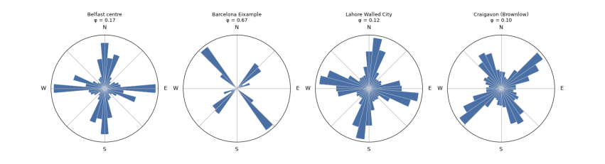
orientation entropy  orientation order φ
Belfast centre                      3.387                0.171
Barcelona Eixample                  2.658                0.665
Lahore Walled City                  3.444                0.123
Craigavon (Brownlow)                3.474                0.097
The roses show the difference at a glance. Barcelona's streets point in two directions, about 45° and 135°, because Cerdà's grid is turned from north to follow the coast; its orientation order is 0.67. It is not 1 because each block has its corners cut off (the xamfrans), adding short diagonal edges, and because the old city and the Avinguda Diagonal cross the square. Belfast (0.17), Lahore (0.12) and Craigavon (0.10) all point every way. The entropy cannot tell an old organic core from a planned curving suburb, since both are disordered in direction: Lahore and Craigavon score almost the same. A single measure reads one property; telling patterns apart needs several together.
3.3 Circuity and route directness
How far out of the way do streets take you? Circuity is the total length of street edges divided by the total straight-line distance between their end nodes: 1 for straight streets, higher for curving ones. A stronger test is route directness: pick pairs of places at random, find the shortest route along streets with Dijkstra's algorithm (NetworkX shortest_path_length), and divide by the straight-line distance between them. A ratio of 1.3 means walking 30 % further than the crow flies. Grids score about 1.2 to 1.3; cul-de-sac layouts can exceed 1.6.
rng = np.random.default_rng(1)
for name, (G, F) in data.items():
    Gu = ox.convert.to_undirected(G)
    streets.loc[name, "edge circuity"] = ox.stats.circuity_avg(Gu)
    big = Gu.subgraph(max(nx.connected_components(Gu), key=len))
    nodes = np.array(list(big.nodes))
    xy = np.array([[big.nodes[n]["x"], big.nodes[n]["y"]] for n in nodes])
    ratios = []
    while len(ratios) < 300:
        i, j = rng.integers(0, len(nodes), 2)
        crow = np.hypot(*(xy[i] - xy[j]))
        if 400 < crow < 1200:                                   # walks of 5 to 15 minutes
            ratios.append(nx.shortest_path_length(big, nodes[i], nodes[j], weight="length") / crow)
    streets.loc[name, "route directness (median)"] = np.median(ratios)
    streets.loc[name, "routes > 1.5x crow"] = 100 * np.mean(np.array(ratios) > 1.5)
print(streets[["edge circuity", "route directness (median)", "routes > 1.5x crow"]].round(2).to_string())
edge circuity  route directness (median)  routes > 1.5x crow
Belfast centre                 1.06                       1.32               18.33
Barcelona Eixample             1.02                       1.26                4.67
Lahore Walled City             1.07                       1.29               11.67
Craigavon (Brownlow)           1.07                       1.81               84.33
Edge circuity is close to 1 everywhere (1.02 to 1.07): individual streets are nearly straight, even in Lahore. Route directness, measured on the walking graph for 300 random walks of 400 to 1,200 m, separates the places sharply. The median walk in Barcelona is 1.26 times the straight-line distance, in Lahore 1.29 and in Belfast 1.32. In Craigavon it is 1.81, and 84 % of walks are more than 1.5 times as long as the crow flies, against 5 % in Barcelona. That is the cost of cul-de-sacs for people on foot: the house across the fence may be ten minutes away. Lahore's crooked lanes still give fairly direct routes because there are so many of them; what matters for walking is the choice of paths, not how straight each one is.
3.4 Centrality: which streets matter most
Some streets carry more through-movement than others because of where they sit in the network, not because of what is on them. Betweenness centrality of a node is the share of all shortest paths between other pairs of nodes that pass through it. High-betweenness streets are the natural main streets: where shops survive and traffic gathers. Closeness centrality is the inverse of the average distance to every other node: high in the middle, low at the edges. Computing betweenness exactly is slow for big graphs, so we estimate it from 400 sampled sources (k=400).
fig, axes = plt.subplots(1, 4, figsize=(14, 4))
for ax, (name, G) in zip(axes, drive.items()):
    Gu = ox.convert.to_undirected(G)
    bc = nx.betweenness_centrality(Gu, k=min(400, len(Gu)), weight="length", seed=1)
    vals = np.array(list(bc.values()))
    top = np.sort(vals)[::-1]
    streets.loc[name, "betweenness: top 5% share"] = top[: max(1, len(top) // 20)].sum() / top.sum()
    mx = max(vals.max(), 1e-12)
    nc = [plt.cm.inferno_r(0.15 + 0.85 * bc[n] / mx) for n in Gu.nodes]
    ns = [1 + 40 * bc[n] / mx for n in Gu.nodes]
    ox.plot_graph(Gu, ax=ax, node_size=ns, node_color=nc, node_zorder=2, edge_color="#ccc", edge_linewidth=0.4,
                  show=False, close=False, bgcolor="white")
    ax.set_title(name, fontsize=10)
plt.tight_layout(); plt.show()
print(streets[["betweenness: top 5% share"]].round(2).to_string())
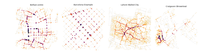
betweenness: top 5% share
Belfast centre                             0.26
Barcelona Eixample                         0.16
Lahore Walled City                         0.40
Craigavon (Brownlow)                       0.45
On the maps, larger and darker nodes carry the most shortest paths. The table gives the share of all betweenness held by the top 5 % of nodes: a measure of how concentrated movement is. In Barcelona it is lowest (16 %): in a regular grid many routes are equally short, so movement spreads over many streets. In Lahore (40 %) and Craigavon (45 %) a few links carry most through-movement: the bazaar spines of the Walled City, and the distributor road of the new town. The same number means different things: in Lahore the busy spines are lined with shops, which is the old logic of the bazaar; in Craigavon they are roads designed to carry cars past homes.