The whole guide on one page
1. Before you start
A good teacher works towards not being needed. This guide does not hand you conclusions about cities; it gives you the means to ask your own questions of the place you live, and to answer them with evidence you can check. You will learn to read a neighbourhood the way urban morphologists do: its streets as a network, its buildings as grain and density, its everyday places as access. Every measure is computed from open data in a notebook you run yourself, explained in words, shown on a map or chart, and accompanied by what it cannot tell you.
Four places are compared throughout, chosen because they were made in very different ways: the centre of Belfast, a port city grown over four centuries; the Eixample of Barcelona, planned on a grid by Ildéfons Cerdà in 1859; the Walled City of Lahore, a dense pre-modern fabric; and Brownlow in Craigavon, a new town of the 1970s laid out around roads and cul-de-sacs.
1.1 Two ways in
-
The Urban form explorer (ahmadammar.github.io/urban-form-explorer) is a web page: pan to any place in the world, zoom in to a neighbourhood, press Analyse this view, and read its streets, buildings, access and indices, each linked to its definition. Nothing to install.
-
The notebook in this guide does the same analyses step by step in Python, so you see and can change every calculation. Open the Notebooks page and choose Open in Colab, or on your own computer:
conda create -n urban python=3.12
conda activate urban
pip install osmnx momepy scikit-learn matplotlib jupyterlab
jupyter lab
Boxes labelled In [n] are code and Out [n] what it printed or drew. Run the cells in order. The first run downloads data from OpenStreetMap’s public servers and keeps a copy in data/cache, so later runs are fast and work offline.
1.2 Setup
This notebook teaches you to read a neighbourhood from open data: its streets, blocks, buildings and everyday places, measured with the same methods urban researchers use. It compares four places with very different histories: the centre of Belfast, Barcelona's planned Eixample, the Walled City of Lahore and the new town of Craigavon. You can then point it at your own street by changing one line.
Libraries: OSMnx downloads OpenStreetMap data and turns streets into a graph; NetworkX does the graph mathematics (shortest paths, centrality); GeoPandas holds buildings and places as tables with shapes; momepy measures urban form; matplotlib draws. In Colab the first cell installs what is missing.
import importlib.util, subprocess, sys
for pkg in ("osmnx", "momepy"):
    if importlib.util.find_spec(pkg) is None:
        subprocess.run([sys.executable, "-m", "pip", "install", "-q", pkg], check=True)
import warnings
warnings.filterwarnings("ignore")
from pathlib import Path
import math
import numpy as np
import pandas as pd
import geopandas as gpd
import networkx as nx
import osmnx as ox
import momepy
import matplotlib.pyplot as plt

Path("data").mkdir(exist_ok=True)
ox.settings.use_cache = True
ox.settings.cache_folder = "data/cache"
ox.settings.log_console = False
plt.rcParams.update({"figure.dpi": 100})
print("osmnx", ox.__version__, "| networkx", nx.__version__, "| momepy", momepy.__version__)

#### The four places: (latitude, longitude) of a centre point. Change or add your own here.
PLACES = {
    "Belfast centre": (54.5973, -5.9301),
    "Barcelona Eixample": (41.3917, 2.1649),
    "Lahore Walled City": (31.5820, 74.3150),
    "Craigavon (Brownlow)": (54.4475, -6.3870),
}
RADIUS = 800          # metres: each study area is the square 1.6 km across around the point
osmnx 2.1.2 | networkx 3.7 | momepy 1.0.0
2. A primer in urban form
2.1 What urban form is
Urban form, or urban morphology, is the physical shape of a settlement: how its streets, plots, blocks and buildings are arranged. The idea is old. The geographer M. R. G. Conzen, studying Alnwick in 1960, split a town plan into three layers that change at different speeds: the street system (slowest: streets last for centuries), the plot pattern (land ownership parcels) and the buildings (fastest: rebuilt every few decades). The Italian school (Muratori, Caniggia) read building types and how they grow. Space syntax (Hillier and Hanson, 1984) studied how the configuration of streets shapes movement.
Today these ideas are measured. A street network is a graph: junctions are nodes, street segments edges. Buildings are polygons with areas, perimeters and heights. From these come numbers that can be compared between any two places on Earth, and that is what this notebook does. A few words used throughout:
-
Urban fabric: the texture made by streets, blocks and buildings together, as you see it on a map.
-
Block: land surrounded by streets. Grain: fine grain means many small blocks and buildings; coarse grain few large ones.
-
Permeability: how many ways there are through an area on foot. Connectivity: how well streets join up.
-
Density: a quantity per area: buildings, floor space, people, junctions.
Numbers do not replace walking a street. They let you ask sharper questions of it: why is this place more walkable than that one, what changed and when, what is missing. Each measure below comes with how to read it and what it cannot tell you.
2.2 Three street patterns
Most street networks are mixtures of three ideal patterns (Figure 2.1). Keep them in mind: each measure in the next chapters separates them in a different way.
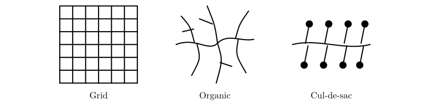
Figure 2.1. Three ideal street patterns. The grid has many four-way junctions, two dominant directions and short, direct routes. The organic pattern, grown over time, has three-way junctions, every direction and moderately direct routes. The cul-de-sac pattern feeds dead ends from a curving distributor road: few junctions and long, indirect routes on foot unless footpaths cut through.
The grid is old: Hippodamus of Miletus planned one in the fifth century BC, Roman camps were grids, and so are Mohenjo-daro, Manhattan and Cerdà’s Barcelona. Organic fabrics grow plot by plot along paths and are typical of pre-modern cores such as Lahore’s Walled City. The cul-de-sac layout belongs to twentieth-century planning that separated cars from homes, as in new towns like Craigavon. None is simply good or bad: grids are legible and easy to walk but can carry through-traffic everywhere; cul-de-sacs are quiet but make short trips long.
2.3 Getting the data
OpenStreetMap (OSM) is a map of the world made by volunteers, free to use under the Open Database Licence. It stores three kinds of element: nodes (points with a latitude and longitude), ways (ordered lists of nodes: streets, building outlines) and relations (groups). Each carries tags, key = value pairs that say what it is: highway=residential, building=yes, building:levels=4, amenity=school. Everything we measure depends on these tags, so their completeness varies by place and must always be checked.
OSMnx asks the Overpass API for the data within a distance of a point and returns a street graph (for walking, network_type="walk", which includes footpaths) and tables of features (buildings, amenities). The graph is projected to a local metric coordinate system (UTM) so that lengths come out in metres.
We download two graphs for each place. The walking graph includes footpaths, and in cities where pavements and crossings are mapped as separate ways it splits every street into many short pieces, so it suits questions about walking (route directness, access) but exaggerates junction counts. The street graph (drive_service: roads and service lanes) describes the layout of streets themselves and is used for structure, orientation and centrality.
SERVERS = ["https://overpass-api.de/api", "https://overpass.private.coffee/api", "https://maps.mail.ru/osm/tools/overpass/api"]


def patient(fn, *args, **kw):
    """Public Overpass servers are shared and sometimes busy: retry with growing waits, trying each server in turn."""
    import time
    for attempt in range(8):
        ox.settings.overpass_url = SERVERS[attempt % len(SERVERS)]
        try:
            return fn(*args, **kw)
        except Exception as e:
            if "No data elements" in str(e):
                raise
            time.sleep(min(60, 5 * 2 ** (attempt // len(SERVERS))))
    raise RuntimeError("Overpass servers busy; run the cell again later")


def fetch(name, latlon):
    G = patient(ox.graph_from_point, latlon, dist=RADIUS, dist_type="bbox", network_type="walk", simplify=True)
    G = ox.project_graph(G)
    tags = {"building": True, "amenity": True, "shop": True, "leisure": ["park", "playground"],
            "public_transport": "platform", "highway": "bus_stop", "railway": ["station", "tram_stop"]}
    F = patient(ox.features_from_point, latlon, tags, dist=RADIUS)
    F = F.to_crs(G.graph["crs"])
    D = ox.project_graph(patient(ox.graph_from_point, latlon, dist=RADIUS, dist_type="bbox", network_type="drive_service"),
                         to_crs=G.graph["crs"])
    return G, F, D


data, drive = {}, {}
for name, latlon in PLACES.items():
    G, F, D = fetch(name, latlon)
    data[name], drive[name] = (G, F), D
    nb = int(F["building"].notna().sum()) if "building" in F else 0
    print(f"{name:22s} walk graph: {G.number_of_nodes():5d} nodes  street graph: {D.number_of_nodes():5d} nodes  "
          f"buildings {nb:5d}  other features {len(F) - nb:4d}")

fig, axes = plt.subplots(1, 4, figsize=(14, 4))
for ax, (name, (G, F)) in zip(axes, data.items()):
    b = F[F["building"].notna()] if "building" in F else F.iloc[:0]
    b[b.geom_type.isin(["Polygon", "MultiPolygon"])].plot(ax=ax, color="#b55", linewidth=0)
    ox.plot_graph(drive[name], ax=ax, node_size=0, edge_color="#333", edge_linewidth=0.5, show=False, close=False, bgcolor="white")
    ax.set_title(name, fontsize=10)
plt.tight_layout(); plt.show()
Belfast centre         walk graph:  2423 nodes  street graph:  1019 nodes  buildings  3317  other features 1424
Barcelona Eixample     walk graph:  2324 nodes  street graph:   315 nodes  buildings  3368  other features 4163
Lahore Walled City     walk graph:  4408 nodes  street graph:  3745 nodes  buildings   471  other features  212
Craigavon (Brownlow)   walk graph:  1571 nodes  street graph:  1020 nodes  buildings   881  other features  418
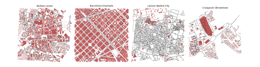
The printout counts what was downloaded for each 1.6 km square. The two graphs differ most in Barcelona: 2,324 nodes for walking but only 315 for streets, because pavements and crossings there are mapped as separate ways. Belfast and Barcelona each have over 3,300 buildings, while the Walled City of Lahore, one of the densest places in South Asia, has only 470. That is not the city; it is the map. Most of Lahore's buildings have not yet been traced in OpenStreetMap, so every building measure for Lahore below is about the mapped part only, a lesson in checking coverage before believing a number. The maps show the street graph in black over mapped buildings in red: Barcelona's grid of square blocks, Belfast's mixture, Lahore's dense mesh of lanes with few buildings drawn, and Craigavon's loops and branches.
The measures in this guide follow published methods: OSMnx for building and measuring networks (Boeing 2017, 2018), street orientation entropy (Boeing 2019), the Spacematrix for density (Berghauser Pont and Haupt 2010), and momepy for building morphometrics (Fleischmann 2019). The layered reading of the town plan goes back to Conzen (1960), and the study of street configuration to Hillier and Hanson (1984).
3. Streets as a network
Streets are the slowest-changing layer of a city and decide how people move through it. This chapter turns them into a graph and reads it four ways: how dense and connected it is, which way it points, how direct its routes are, and which streets matter most.
3.1 Streets as a graph
Here we use the street graph. In it each node is a junction or a dead end, each edge a street segment between two nodes. The number of streets meeting at a node is its degree; OSMnx counts streets per node without double-counting two-way edges. From these come the basic network measures:
-
Intersection density: junctions (nodes with 3 or more streets) per km². Higher means smaller blocks and more choice of route. Values above about 100 per km² are typical of walkable centres.
-
Street density: km of street per km².
-
Mean streets per node: 4 in a perfect grid, about 3 where T-junctions dominate, lower where there are many dead ends.
-
Share of dead ends (degree 1): cul-de-sacs; high in post-war suburbs.
-
Mean edge length: a proxy for block size.
def area_km2(G):
    xs = [d["x"] for _, d in G.nodes(data=True)]; ys = [d["y"] for _, d in G.nodes(data=True)]
    return (max(xs) - min(xs)) * (max(ys) - min(ys)) / 1e6


rows = {}
for name, G in drive.items():
    A = area_km2(G)
    spn = pd.Series(dict(G.nodes(data="street_count")))
    Gu = ox.convert.to_undirected(G)
    L = sum(d["length"] for *_, d in Gu.edges(data=True)) / 1000
    rows[name] = {
        "area km²": A,
        "intersections per km²": (spn >= 3).sum() / A,
        "street km per km²": L / A,
        "mean streets per node": spn.mean(),
        "dead ends %": 100 * (spn == 1).mean(),
        "4-way %": 100 * (spn == 4).mean(),
        "mean edge length m": np.mean([d["length"] for *_, d in Gu.edges(data=True)]),
    }
streets = pd.DataFrame(rows).T
print(streets.round(1).to_string())
area km²  intersections per km²  street km per km²  mean streets per node  dead ends %  4-way %  mean edge length m
Belfast centre             2.6                  275.0               21.7                    2.5         28.9      9.7                44.9
Barcelona Eixample         2.5                  117.2               17.3                    3.5          5.7     51.4                86.6
Lahore Walled City         2.6                  935.0               41.1                    2.3         36.1      4.4                24.4
Craigavon (Brownlow)       2.4                  235.9               14.5                    2.2         43.6      2.7                32.2
Read the table column by column. Streets per node separates the patterns: 3.5 in the Eixample, where half of all nodes (51 %) are four-way crossings, against 2.2 to 2.5 elsewhere. Dead ends are rare in Barcelona (6 %) and common in Craigavon (44 %), the cul-de-sac signature. Lahore's Walled City has by far the most junctions, 935 per km², and the shortest street segments (24 m): its lanes (galis) branch and meet every few metres, and over a third (36 %) end blindly in courtyards, which is the classic organic pattern. Barcelona has the fewest junctions (117 per km²) and the longest segments (87 m) because its blocks are large, 113 m squares. So intersection density alone does not mean walkable: a fine organic mesh and a coarse grid can both work well on foot, and a suburb can have many junctions that all lead to dead ends.
3.2 Orientation and order
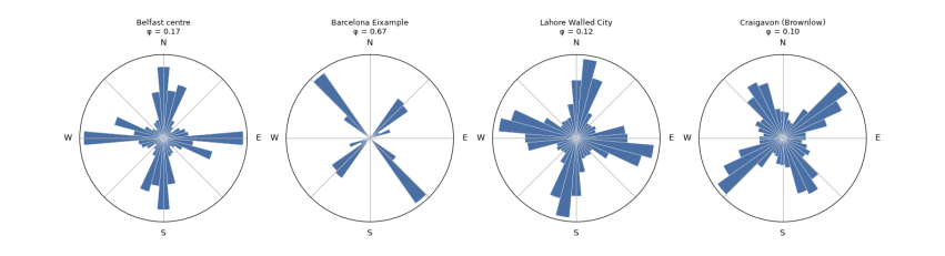
Which way do the streets point? For each edge take its compass bearing (0° north, 90° east), count both directions (a street running north also runs south), and gather them into 36 bins of 10°. A rose diagram shows the result: a grid gives four petals; an unplanned or curving fabric gives a near circle.
Orientation entropy (Boeing 2019) measures the disorder: H = −Σ p_i ln p_i over the 36 bins. A perfect four-way grid has H = ln 4 ≈ 1.386; streets spread evenly over all directions have H = ln 36 ≈ 3.584. Orientation order rescales it from 0 (disorder) to 1 (perfect grid): φ = 1 − ((H − 1.386)/(3.584 − 1.386))².
def orientation(G):
    Gu = ox.convert.to_undirected(ox.bearing.add_edge_bearings(ox.project_graph(G, to_latlong=True)))
    b = np.array([d["bearing"] for *_, d in Gu.edges(data=True) if not np.isnan(d.get("bearing", np.nan))])
    w = np.array([d["length"] for *_, d in Gu.edges(data=True) if not np.isnan(d.get("bearing", np.nan))])
    both = np.concatenate([b, (b + 180) % 360]); ww = np.concatenate([w, w])
    counts, _ = np.histogram((both + 5) % 360, bins=36, range=(0, 360), weights=ww)   # bins centred on 0, 10, ...
    p = counts / counts.sum()
    H = -(p[p > 0] * np.log(p[p > 0])).sum()
    phi = 1 - ((H - np.log(4)) / (np.log(36) - np.log(4))) ** 2
    return counts, H, phi


fig, axes = plt.subplots(1, 4, figsize=(14, 3.8), subplot_kw={"projection": "polar"})
for ax, (name, G) in zip(axes, drive.items()):
    counts, H, phi = orientation(G)
    streets.loc[name, "orientation entropy"] = H
    streets.loc[name, "orientation order φ"] = phi
    th = np.radians(np.arange(0, 360, 10))
    ax.bar(th, counts / counts.max(), width=np.radians(10), color="#4a6fa5", edgecolor="white", linewidth=0.3)
    ax.set_theta_zero_location("N"); ax.set_theta_direction(-1); ax.set_yticks([]); ax.set_xticklabels(["N", "", "E", "", "S", "", "W", ""])
    ax.set_title(f"{name}\nφ = {phi:.2f}", fontsize=9)
plt.tight_layout(); plt.show()
print(streets[["orientation entropy", "orientation order φ"]].round(3).to_string())
orientation entropy  orientation order φ
Belfast centre                      3.387                0.171
Barcelona Eixample                  2.658                0.665
Lahore Walled City                  3.444                0.123
Craigavon (Brownlow)                3.474                0.097
The roses show the difference at a glance. Barcelona's streets point in two directions, about 45° and 135°, because Cerdà's grid is turned from north to follow the coast; its orientation order is 0.67. It is not 1 because each block has its corners cut off (the xamfrans), adding short diagonal edges, and because the old city and the Avinguda Diagonal cross the square. Belfast (0.17), Lahore (0.12) and Craigavon (0.10) all point every way. The entropy cannot tell an old organic core from a planned curving suburb, since both are disordered in direction: Lahore and Craigavon score almost the same. A single measure reads one property; telling patterns apart needs several together.
3.3 Circuity and route directness
How far out of the way do streets take you? Circuity is the total length of street edges divided by the total straight-line distance between their end nodes: 1 for straight streets, higher for curving ones. A stronger test is route directness: pick pairs of places at random, find the shortest route along streets with Dijkstra's algorithm (NetworkX shortest_path_length), and divide by the straight-line distance between them. A ratio of 1.3 means walking 30 % further than the crow flies. Grids score about 1.2 to 1.3; cul-de-sac layouts can exceed 1.6.
rng = np.random.default_rng(1)
for name, (G, F) in data.items():
    Gu = ox.convert.to_undirected(G)
    streets.loc[name, "edge circuity"] = ox.stats.circuity_avg(Gu)
    big = Gu.subgraph(max(nx.connected_components(Gu), key=len))
    nodes = np.array(list(big.nodes))
    xy = np.array([[big.nodes[n]["x"], big.nodes[n]["y"]] for n in nodes])
    ratios = []
    while len(ratios) < 300:
        i, j = rng.integers(0, len(nodes), 2)
        crow = np.hypot(*(xy[i] - xy[j]))
        if 400 < crow < 1200:                                   # walks of 5 to 15 minutes
            ratios.append(nx.shortest_path_length(big, nodes[i], nodes[j], weight="length") / crow)
    streets.loc[name, "route directness (median)"] = np.median(ratios)
    streets.loc[name, "routes > 1.5x crow"] = 100 * np.mean(np.array(ratios) > 1.5)
print(streets[["edge circuity", "route directness (median)", "routes > 1.5x crow"]].round(2).to_string())
edge circuity  route directness (median)  routes > 1.5x crow
Belfast centre                 1.06                       1.32               18.33
Barcelona Eixample             1.02                       1.26                4.67
Lahore Walled City             1.07                       1.29               11.67
Craigavon (Brownlow)           1.07                       1.81               84.33
Edge circuity is close to 1 everywhere (1.02 to 1.07): individual streets are nearly straight, even in Lahore. Route directness, measured on the walking graph for 300 random walks of 400 to 1,200 m, separates the places sharply. The median walk in Barcelona is 1.26 times the straight-line distance, in Lahore 1.29 and in Belfast 1.32. In Craigavon it is 1.81, and 84 % of walks are more than 1.5 times as long as the crow flies, against 5 % in Barcelona. That is the cost of cul-de-sacs for people on foot: the house across the fence may be ten minutes away. Lahore's crooked lanes still give fairly direct routes because there are so many of them; what matters for walking is the choice of paths, not how straight each one is.
3.4 Centrality: which streets matter most
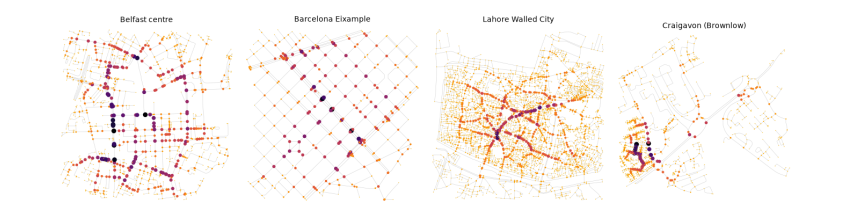
Some streets carry more through-movement than others because of where they sit in the network, not because of what is on them. Betweenness centrality of a node is the share of all shortest paths between other pairs of nodes that pass through it. High-betweenness streets are the natural main streets: where shops survive and traffic gathers. Closeness centrality is the inverse of the average distance to every other node: high in the middle, low at the edges. Computing betweenness exactly is slow for big graphs, so we estimate it from 400 sampled sources (k=400).
fig, axes = plt.subplots(1, 4, figsize=(14, 4))
for ax, (name, G) in zip(axes, drive.items()):
    Gu = ox.convert.to_undirected(G)
    bc = nx.betweenness_centrality(Gu, k=min(400, len(Gu)), weight="length", seed=1)
    vals = np.array(list(bc.values()))
    top = np.sort(vals)[::-1]
    streets.loc[name, "betweenness: top 5% share"] = top[: max(1, len(top) // 20)].sum() / top.sum()
    mx = max(vals.max(), 1e-12)
    nc = [plt.cm.inferno_r(0.15 + 0.85 * bc[n] / mx) for n in Gu.nodes]
    ns = [1 + 40 * bc[n] / mx for n in Gu.nodes]
    ox.plot_graph(Gu, ax=ax, node_size=ns, node_color=nc, node_zorder=2, edge_color="#ccc", edge_linewidth=0.4,
                  show=False, close=False, bgcolor="white")
    ax.set_title(name, fontsize=10)
plt.tight_layout(); plt.show()
print(streets[["betweenness: top 5% share"]].round(2).to_string())
betweenness: top 5% share
Belfast centre                             0.26
Barcelona Eixample                         0.16
Lahore Walled City                         0.40
Craigavon (Brownlow)                       0.45
On the maps, larger and darker nodes carry the most shortest paths. The table gives the share of all betweenness held by the top 5 % of nodes: a measure of how concentrated movement is. In Barcelona it is lowest (16 %): in a regular grid many routes are equally short, so movement spreads over many streets. In Lahore (40 %) and Craigavon (45 %) a few links carry most through-movement: the bazaar spines of the Walled City, and the distributor road of the new town. The same number means different things: in Lahore the busy spines are lined with shops, which is the old logic of the bazaar; in Craigavon they are roads designed to carry cars past homes.
4. Buildings: grain and density
Buildings change faster than streets, but they give a place its character: how tall, how close, how joined. This chapter measures density with the Spacematrix and the shape of each building with momepy.
4.1 Grain, density and the Spacematrix
Building footprints give the grain of a place (how big the buildings are) and its density. Berghauser Pont and Haupt's Spacematrix (2010) describes density with three linked numbers:
-
GSI, ground space index or coverage: building footprint area ÷ land area.
-
FSI, floor space index: total floor area (footprint × floors) ÷ land area.
-
L, mean number of floors = FSI ÷ GSI. And OSR, open space ratio = (1 − GSI) ÷ FSI: open ground per unit of floor.
Low-rise sprawl has low GSI and low FSI; a dense historic centre has high GSI and middling FSI; towers in a park have low GSI and high FSI. Floors come from the OSM tags building:levels, or height ÷ 3 m; where neither is tagged we must assume a value, and the share assumed is reported.
def floors(row):
    for key in ("building:levels",):
        if key in row and pd.notna(row[key]):
            try:
                return float(str(row[key]).split(";")[0]), True
            except ValueError:
                pass
    if "height" in row and pd.notna(row["height"]):
        try:
            return max(1.0, round(float(str(row["height"]).replace("m", "").split(";")[0]) / 3)), True
        except ValueError:
            pass
    return np.nan, False


bstats, blds = {}, {}
for name, (G, F) in data.items():
    b = F[F["building"].notna() & F.geom_type.isin(["Polygon", "MultiPolygon"])].copy()
    fl = b.apply(floors, axis=1, result_type="expand"); b["floors"], b["tagged"] = fl[0], fl[1].astype(bool)
    default = b.loc[b.tagged, "floors"].median() if b.tagged.mean() > 0.2 else 2.0
    b["floors_used"] = b["floors"].fillna(default)
    b["area"] = b.area
    blds[name] = b
    land = (2 * RADIUS) ** 2
    gsi = b.area.sum() / land
    fsi = (b.area * b.floors_used).sum() / land
    bstats[name] = {"buildings": len(b), "per hectare": len(b) / (land / 1e4), "median footprint m²": b.area.median(),
                    "floors tagged %": 100 * b.tagged.mean(), "assumed floors": default,
                    "GSI": gsi, "FSI": fsi, "L floors": fsi / gsi, "OSR": (1 - gsi) / fsi}
bstats = pd.DataFrame(bstats).T
print(bstats.round(2).to_string())

fig, ax = plt.subplots(figsize=(6, 4.5))
offsets = {"Belfast centre": (6, 4), "Barcelona Eixample": (-110, 4), "Lahore Walled City": (6, 10), "Craigavon (Brownlow)": (6, -12)}
for name, r in bstats.iterrows():
    ax.scatter(r.GSI, r.FSI, s=60); ax.annotate(name, (r.GSI, r.FSI), fontsize=8, xytext=offsets.get(name, (4, 4)), textcoords="offset points")
g = np.linspace(0.01, 0.8, 50)
for L in (1, 2, 4, 8):
    ax.plot(g, g * L, color="grey", lw=0.6, ls=":")
    xl = min(0.8, 4.6 / L); ax.text(xl, xl * L, f" {L} floors", fontsize=7, color="grey", va="bottom")
ax.set_xlim(0, 0.9); ax.set_ylim(0, 5); ax.set_xlabel("GSI (coverage)"); ax.set_ylabel("FSI (floor space index)")
ax.set_title("Spacematrix: the four places"); plt.tight_layout(); plt.show()
buildings  per hectare  median footprint m²  floors tagged %  assumed floors   GSI   FSI  L floors   OSR
Belfast centre           3316.0        12.95                52.71            33.87             2.0  0.33  1.01      3.07  0.67
Barcelona Eixample       3353.0        13.10               345.80            59.86             7.0  0.59  4.23      7.14  0.10
Lahore Walled City        470.0         1.84                89.30             1.06             2.0  0.05  0.11      2.00  8.65
Craigavon (Brownlow)      881.0         3.44               111.07             0.91             2.0  0.13  0.25      1.96  3.55
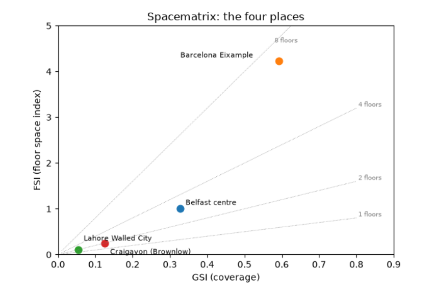
The Spacematrix table and chart place the four areas. The Eixample covers 59 % of its land with buildings (GSI 0.59), at a median footprint of 346 m² (whole blocks of joined apartment buildings) and a floor space index of 4.2: about seven floors on average, with 60 % of buildings carrying a floors tag. Little open ground remains per unit of floor (OSR 0.10). Central Belfast has a third of its land covered, an FSI of 1.0 and about three floors; floors are tagged for a third of buildings, so the rest assume the tagged median of 2. Craigavon is low-rise and open: GSI 0.13, FSI 0.25, under 2 floors. Lahore's figures (GSI 0.05) are an artefact: with most buildings unmapped and almost no floors tagged (1 %), its true coverage is far higher. Always read the 'floors tagged %' and building count before the density.
4.2 Morphometrics: the shape of each building
momepy measures many properties of individual elements. Three useful ones for buildings:
-
Elongation: the ratio of the short to the long side of the smallest rotated rectangle around the footprint (1 = square, near 0 = long and thin, like a terrace row).
-
Circular compactness: footprint area ÷ area of the smallest enclosing circle (1 for a circle, low for L- and courtyard-shaped buildings).
-
Shared walls ratio: the share of the perimeter touching another building. High in terraces and historic cores where buildings are joined; zero for detached houses.
morph = {}
for name, b in blds.items():
    b = b.reset_index(drop=True)
    b = b[b.is_valid & (b.area > 10)].copy()
    b["elongation"] = momepy.elongation(b)
    b["compactness"] = momepy.circular_compactness(b)
    b["shared walls"] = momepy.shared_walls(b) / b.length
    blds[name] = b
    morph[name] = b[["area", "elongation", "compactness", "shared walls"]].median()
    morph[name]["joined to a neighbour %"] = 100 * (b["shared walls"] > 0.05).mean()
morph = pd.DataFrame(morph).T
print(morph.round(2).to_string())

fig, axes = plt.subplots(1, 4, figsize=(14, 4))
for ax, (name, b) in zip(axes, blds.items()):
    b.plot(column="shared walls", ax=ax, cmap="viridis", vmin=0, vmax=0.6, linewidth=0)
    ax.set_title(name, fontsize=10); ax.set_axis_off()
plt.suptitle("Share of each building's perimeter shared with a neighbour (yellow = joined, purple = detached)", fontsize=10)
plt.tight_layout(); plt.show()
area  elongation  compactness  shared walls  joined to a neighbour %
Belfast centre         53.08        0.62         0.54          0.37                    86.55
Barcelona Eixample    346.16        0.47         0.43          0.57                    98.03
Lahore Walled City     89.34        0.65         0.53          0.50                    71.43
Craigavon (Brownlow)  111.09        0.75         0.57          0.00                    29.89
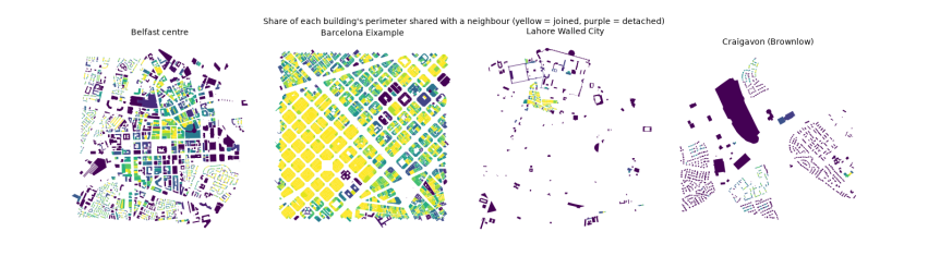
The medians describe a typical building in each place. Barcelona's buildings are large (346 m²) and joined: 98 % share part of their outline with a neighbour, and on average 57 % of a building's perimeter is a party wall. That is the perimeter block: continuous street walls around a courtyard. Belfast's terraces show the same habit at smaller size (53 m², 87 % joined). In Craigavon the median building shares no wall at all, and only 30 % touch a neighbour, mostly semi-detached pairs: detached and semi-detached houses on their own plots. Craigavon's buildings are also the most nearly square (elongation 0.75). The maps show these differences as colour: yellow continuous blocks against purple free-standing houses.
5. Access: what you can reach on foot
Form matters because of what it lets people do. The test used here is the one behind the idea of the 15-minute city: how many kinds of everyday place can you reach within a quarter of an hour’s walk?
5.1 The 15-minute question
Can you reach daily needs on foot? Take the centre of each study area, find all street nodes within 15 minutes' walk (1,200 m at 80 m a minute) along the network with Dijkstra's algorithm, build the isochrone (the area reachable), and count the everyday places inside it by kind. The walking distance is along streets, not as the crow flies, so a circuitous layout reaches less.
KINDS = {
    "food shop": lambda r: r.get("shop") in ("supermarket", "convenience", "greengrocer", "bakery", "butcher", "general"),
    "school": lambda r: r.get("amenity") in ("school", "kindergarten"),
    "health": lambda r: r.get("amenity") in ("pharmacy", "doctors", "clinic", "hospital", "dentist"),
    "food and drink": lambda r: r.get("amenity") in ("restaurant", "cafe", "fast_food", "pub"),
    "park or play": lambda r: r.get("leisure") in ("park", "playground"),
    "transit stop": lambda r: r.get("highway") == "bus_stop" or r.get("public_transport") == "platform" or r.get("railway") in ("station", "tram_stop"),
    "worship": lambda r: r.get("amenity") == "place_of_worship",
}
access = {}
for name, (G, F) in data.items():
    Gu = ox.convert.to_undirected(G)
    xs = np.array([d["x"] for _, d in Gu.nodes(data=True)]); ys = np.array([d["y"] for _, d in Gu.nodes(data=True)])
    centre = ox.distance.nearest_nodes(Gu, xs.mean(), ys.mean())
    reach = nx.single_source_dijkstra_path_length(Gu, centre, cutoff=1200, weight="length")
    pts = gpd.GeoSeries(gpd.points_from_xy([Gu.nodes[n]["x"] for n in reach], [Gu.nodes[n]["y"] for n in reach]), crs=F.crs)
    iso = pts.union_all().convex_hull.buffer(50)
    P = F[F.representative_point().within(iso)]
    rec = {k: int(sum(bool(f(r)) for r in P.to_dict("records"))) for k, f in KINDS.items()}
    rec["isochrone km²"] = iso.area / 1e6
    rec["kinds present (of 7)"] = sum(rec[k] > 0 for k in KINDS)
    access[name] = rec
access = pd.DataFrame(access).T
print(access.round(2).to_string())
food shop  school  health  food and drink  park or play  transit stop  worship  isochrone km²  kinds present (of 7)
Belfast centre             41.0     3.0    11.0           234.0          11.0          85.0     19.0           2.51                   7.0
Barcelona Eixample        203.0    29.0   119.0           946.0          23.0         178.0     17.0           2.80                   7.0
Lahore Walled City          1.0     8.0     5.0            11.0          29.0           1.0    110.0           2.59                   7.0
Craigavon (Brownlow)        5.0     0.0     0.0             8.0           0.0          10.0      2.0           1.47                   4.0
From the centre of each area, the reachable area in 15 minutes is about 2.5 to 2.8 km² in the three older places but only 1.5 km² in Craigavon, because its routes are indirect. Barcelona's isochrone holds 203 food shops, 119 health places and 946 places to eat or drink: everyday needs on every block. Central Belfast has all seven kinds too. Craigavon's centre reaches only four of the seven kinds, with no school, health place or park mapped within the walk. Lahore reaches all seven, with 110 places of worship, but only one food shop, which is implausible for one of the busiest bazaars in Pakistan and again reflects mapping, not reality. Counts are only as good as the tags: check a few against what you know.
6. Neighbourhood types
The previous chapters compared four whole places. Within one city, fabric changes from street to street. This chapter measures many small cells of Belfast and lets the data group them into types, which you then name and question.
6.1 Neighbourhood types from the data
Can the computer tell kinds of fabric apart? Divide one larger area into a grid of 250 m cells, measure each cell (intersections, building count and coverage, median footprint, shared walls, dead-end share), standardise the measures so each has mean 0 and standard deviation 1, and group similar cells with k-means clustering. The clusters are not labelled by the computer: you name them by reading their average values and looking at the map. This is how urban-form typologies (for example the momepy-based classifications of whole countries) are built.
from sklearn.cluster import KMeans
from sklearn.preprocessing import StandardScaler

city_pt, city_r = (54.5900, -5.9300), 2500                       # Belfast, 5 km across
Gc = ox.project_graph(patient(ox.graph_from_point, city_pt, dist=city_r, dist_type="bbox", network_type="drive_service"))
Bc = patient(ox.features_from_point, city_pt, {"building": True}, dist=city_r).to_crs(Gc.graph["crs"])
Bc = Bc[Bc.geom_type.isin(["Polygon", "MultiPolygon"])].reset_index(drop=True)
Bc = Bc[Bc.is_valid].copy()
Bc["sw"] = momepy.shared_walls(Bc) / Bc.length
nodes_c = ox.graph_to_gdfs(Gc, edges=False)
x0, y0, x1, y1 = Bc.total_bounds
size = 250
cells = gpd.GeoDataFrame(geometry=[__import__("shapely").box(x, y, x + size, y + size)
                                   for x in np.arange(x0, x1, size) for y in np.arange(y0, y1, size)], crs=Bc.crs)
cent = Bc.copy(); cent["geometry"] = Bc.representative_point(); cent["a"] = Bc.area
j = gpd.sjoin(cent, cells, predicate="within")
g = j.groupby("index_right")
feat = pd.DataFrame({"buildings": g.size(), "coverage": g["a"].sum() / size ** 2,
                     "median footprint": g["a"].median(), "shared walls": g["sw"].mean()})
jn = gpd.sjoin(nodes_c, cells, predicate="within")
feat["junctions"] = jn[jn.street_count >= 3].groupby("index_right").size()
feat["dead ends"] = jn[jn.street_count == 1].groupby("index_right").size()
feat = feat.fillna(0)
feat = feat[feat.buildings >= 5]
X = StandardScaler().fit_transform(np.log1p(feat))
km = KMeans(n_clusters=5, n_init=20, random_state=0).fit(X)
feat["type"] = km.labels_
summary = feat.groupby("type").median().round(2)
summary["cells"] = feat.groupby("type").size()
print(summary.to_string())

cells_t = cells.join(feat["type"], how="inner")
fig, ax = plt.subplots(figsize=(7, 7))
cells_t.plot(column="type", categorical=True, cmap="Set2", ax=ax, alpha=0.75, legend=True, legend_kwds={"title": "type", "fontsize": 8})
Bc.plot(ax=ax, color="black", linewidth=0, alpha=0.5)
ax.set_axis_off(); ax.set_title("Belfast: 250 m cells grouped into five fabric types"); plt.tight_layout(); plt.show()
buildings  coverage  median footprint  shared walls  junctions  dead ends  cells
type
0         135.5      0.22             51.84          0.35       17.0        9.0    150
1          18.0      0.31            390.06          0.10       14.5        5.5     44
2         316.5      0.32             47.16          0.51       18.0        5.0     70
3          84.0      0.15             54.36          0.26        5.0        3.0     92
4          11.0      0.06            134.96          0.02        2.0        1.0     39
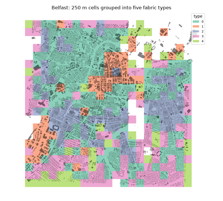
The table gives the median of each measure in each type, and the map shows where the types fall. Reading them, with names we give, not the computer:
-
Type 2, dense terraces: about 316 buildings per cell, small footprints (47 m²) and the most shared walls (0.51): the Victorian terraced streets around the centre.
-
Type 0, terraced and semi-detached housing: fewer buildings (136), still small and partly joined (0.35).
-
Type 3, suburban housing: lower coverage (0.15), few junctions (5 per cell): later, looser estates.
-
Type 1, large buildings: few but big footprints (390 m²) at high coverage (0.31): the commercial centre, retail, hospitals and industry.
-
Type 4, open land with scattered buildings: coverage 0.06: parks, docks, the edges.
The number of types (five) is a choice: try 4 or 7 and see which split is most meaningful. The types come from the data, but their meaning comes from you.
7. Your own neighbourhood
7.1 Reading responsibly
Every number above rests on what volunteers have mapped. Before trusting a figure, ask:
-
Coverage: are all buildings mapped? Compare with satellite imagery for a few blocks. Are floors or heights tagged for most buildings, or are we assuming? (The table in the Buildings section reports this.)
-
Edges: a square study area cuts streets and blocks at its border; measures near the edge are biased.
-
Definitions: a 'walk' network includes footpaths that a 'drive' network lacks; dead ends for cars may be through routes on foot. Say which you used.
-
Population: OSM holds no population counts. Use a census or a gridded product (WorldPop, GHSL) for people per km².
-
The lived city: numbers say nothing of safety, shade, noise, cost, who is welcome. Walk it, talk to people, read its history. Use the numbers to sharpen questions, not to end them.
Questions to take to your own neighbourhood. Change PLACES in the first cell to your street and run everything. Is your area closer to a grid or to an organic pattern, and why (when was it built, by whom, over what)? Which street has the highest betweenness, and is that where the shops are? How many of the seven everyday kinds can you reach in 15 minutes, and which is missing? Which fabric type is your home in, and what would it take to change it?
7.2 The same measures in your browser
The Urban form explorer computes the measures of this guide for any area you choose, with no installation. It fetches OpenStreetMap data from the same public Overpass servers, works in a local metric projection in the browser, and reports streets (density, junctions, dead ends, circuity, route directness, orientation order with a rose diagram), buildings (count, footprints, floors where tagged, GSI, FSI, open space ratio), access (walking distance along streets to the nearest place of each everyday kind) and composite indices for walkability, cyclability and public transport, always shown with their parts. Each figure links to its formula on the methods page, and each analysis reports how much of the area carries the tags it relies on. Use the notebook to understand a measure, and the explorer to apply it widely; when the two disagree, the notebook shows you why.
7.3 What you have learned
-
Urban form has layers that change at different speeds: streets, plots, buildings.
-
OpenStreetMap stores the city as nodes, ways and tagged relations; OSMnx turns streets into a graph.
-
Network measures (intersection density, streets per node, dead ends, orientation order, circuity, route directness, betweenness) describe how a street pattern works for movement.
-
Building measures (GSI, FSI, floors, OSR, elongation, compactness, shared walls) describe grain and density.
-
Network distance, not straight-line distance, decides what you can reach.
-
Clustering many cells by their measures yields fabric types you then name and question.
-
Every figure depends on mapping completeness, which must be checked and reported.
References
Berghauser Pont, Meta, and Per Haupt. 2010. Spacematrix: Space, Density and Urban Form. NAi Publishers.
Boeing, Geoff. 2017. “OSMnx: New Methods for Acquiring, Constructing, Analyzing, and Visualizing Complex Street Networks.” Computers, Environment and Urban Systems 65: 126–39. https://doi.org/10.1016/j.compenvurbsys.2017.05.004.
Boeing, Geoff. 2018. “A Multi-Scale Analysis of 27,000 Urban Street Networks: Every US City, Town, Urbanized Area, and Zillow Neighborhood.” Environment and Planning B: Urban Analytics and City Science 47 (4): 590–608. https://doi.org/10.1177/2399808318784595.
Boeing, Geoff. 2019. “Urban Spatial Order: Street Network Orientation, Configuration, and Entropy.” Applied Network Science 4 (1). https://doi.org/10.1007/s41109-019-0189-1.
Conzen, M. R. G. 1960. Alnwick, Northumberland: A Study in Town-Plan Analysis. Institute of British Geographers Publication 27. George Philip.
Fleischmann, Martin. 2019. “Momepy: Urban Morphology Measuring Toolkit.” Journal of Open Source Software 4 (43): 1807. https://doi.org/10.21105/joss.01807.
Hillier, Bill, and Julienne Hanson. 1984. The Social Logic of Space. Cambridge University Press. https://doi.org/10.1017/cbo9780511597237.