6. Neighbourhood types
The previous chapters compared four whole places. Within one city, fabric changes from street to street. This chapter measures many small cells of Belfast and lets the data group them into types, which you then name and question.
6.1 Neighbourhood types from the data
Can the computer tell kinds of fabric apart? Divide one larger area into a grid of 250 m cells, measure each cell (intersections, building count and coverage, median footprint, shared walls, dead-end share), standardise the measures so each has mean 0 and standard deviation 1, and group similar cells with k-means clustering. The clusters are not labelled by the computer: you name them by reading their average values and looking at the map. This is how urban-form typologies (for example the momepy-based classifications of whole countries) are built.
from sklearn.cluster import KMeans
from sklearn.preprocessing import StandardScaler

city_pt, city_r = (54.5900, -5.9300), 2500                       # Belfast, 5 km across
Gc = ox.project_graph(patient(ox.graph_from_point, city_pt, dist=city_r, dist_type="bbox", network_type="drive_service"))
Bc = patient(ox.features_from_point, city_pt, {"building": True}, dist=city_r).to_crs(Gc.graph["crs"])
Bc = Bc[Bc.geom_type.isin(["Polygon", "MultiPolygon"])].reset_index(drop=True)
Bc = Bc[Bc.is_valid].copy()
Bc["sw"] = momepy.shared_walls(Bc) / Bc.length
nodes_c = ox.graph_to_gdfs(Gc, edges=False)
x0, y0, x1, y1 = Bc.total_bounds
size = 250
cells = gpd.GeoDataFrame(geometry=[__import__("shapely").box(x, y, x + size, y + size)
                                   for x in np.arange(x0, x1, size) for y in np.arange(y0, y1, size)], crs=Bc.crs)
cent = Bc.copy(); cent["geometry"] = Bc.representative_point(); cent["a"] = Bc.area
j = gpd.sjoin(cent, cells, predicate="within")
g = j.groupby("index_right")
feat = pd.DataFrame({"buildings": g.size(), "coverage": g["a"].sum() / size ** 2,
                     "median footprint": g["a"].median(), "shared walls": g["sw"].mean()})
jn = gpd.sjoin(nodes_c, cells, predicate="within")
feat["junctions"] = jn[jn.street_count >= 3].groupby("index_right").size()
feat["dead ends"] = jn[jn.street_count == 1].groupby("index_right").size()
feat = feat.fillna(0)
feat = feat[feat.buildings >= 5]
X = StandardScaler().fit_transform(np.log1p(feat))
km = KMeans(n_clusters=5, n_init=20, random_state=0).fit(X)
feat["type"] = km.labels_
summary = feat.groupby("type").median().round(2)
summary["cells"] = feat.groupby("type").size()
print(summary.to_string())

cells_t = cells.join(feat["type"], how="inner")
fig, ax = plt.subplots(figsize=(7, 7))
cells_t.plot(column="type", categorical=True, cmap="Set2", ax=ax, alpha=0.75, legend=True, legend_kwds={"title": "type", "fontsize": 8})
Bc.plot(ax=ax, color="black", linewidth=0, alpha=0.5)
ax.set_axis_off(); ax.set_title("Belfast: 250 m cells grouped into five fabric types"); plt.tight_layout(); plt.show()
buildings  coverage  median footprint  shared walls  junctions  dead ends  cells
type
0         135.5      0.22             51.84          0.35       17.0        9.0    150
1          18.0      0.31            390.06          0.10       14.5        5.5     44
2         316.5      0.32             47.16          0.51       18.0        5.0     70
3          84.0      0.15             54.36          0.26        5.0        3.0     92
4          11.0      0.06            134.96          0.02        2.0        1.0     39
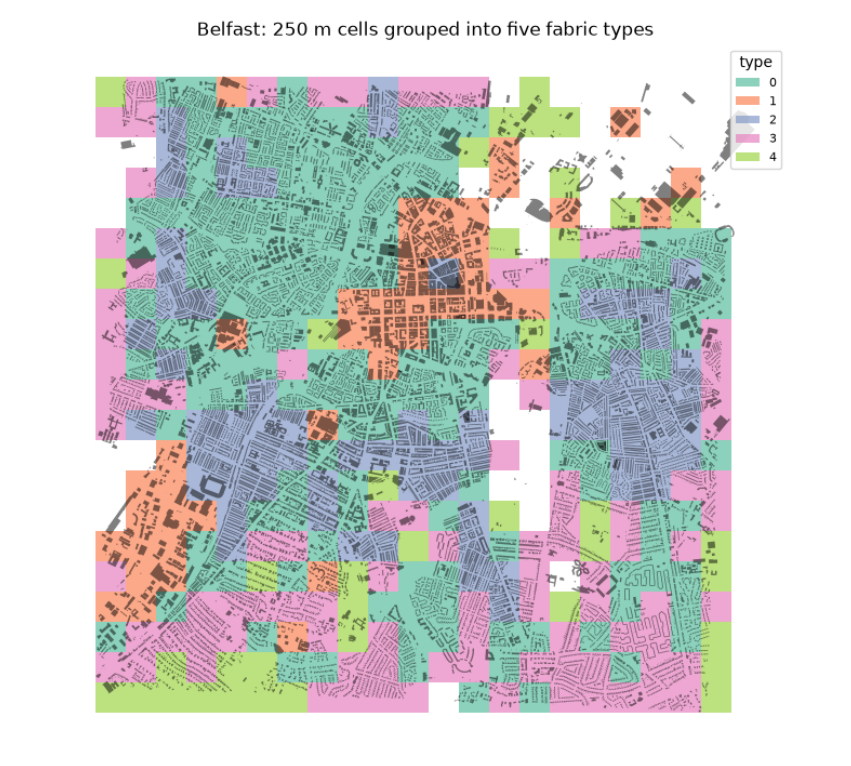
The table gives the median of each measure in each type, and the map shows where the types fall. Reading them, with names we give, not the computer:
-
Type 2, dense terraces: about 316 buildings per cell, small footprints (47 m²) and the most shared walls (0.51): the Victorian terraced streets around the centre.
-
Type 0, terraced and semi-detached housing: fewer buildings (136), still small and partly joined (0.35).
-
Type 3, suburban housing: lower coverage (0.15), few junctions (5 per cell): later, looser estates.
-
Type 1, large buildings: few but big footprints (390 m²) at high coverage (0.31): the commercial centre, retail, hospitals and industry.
-
Type 4, open land with scattered buildings: coverage 0.06: parks, docks, the edges.
The number of types (five) is a choice: try 4 or 7 and see which split is most meaningful. The types come from the data, but their meaning comes from you.