4. Buildings: grain and density
Buildings change faster than streets, but they give a place its character: how tall, how close, how joined. This chapter measures density with the Spacematrix and the shape of each building with momepy.
4.1 Grain, density and the Spacematrix
Building footprints give the grain of a place (how big the buildings are) and its density. Berghauser Pont and Haupt's Spacematrix (2010) describes density with three linked numbers:
-
GSI, ground space index or coverage: building footprint area ÷ land area.
-
FSI, floor space index: total floor area (footprint × floors) ÷ land area.
-
L, mean number of floors = FSI ÷ GSI. And OSR, open space ratio = (1 − GSI) ÷ FSI: open ground per unit of floor.
Low-rise sprawl has low GSI and low FSI; a dense historic centre has high GSI and middling FSI; towers in a park have low GSI and high FSI. Floors come from the OSM tags building:levels, or height ÷ 3 m; where neither is tagged we must assume a value, and the share assumed is reported.
def floors(row):
    for key in ("building:levels",):
        if key in row and pd.notna(row[key]):
            try:
                return float(str(row[key]).split(";")[0]), True
            except ValueError:
                pass
    if "height" in row and pd.notna(row["height"]):
        try:
            return max(1.0, round(float(str(row["height"]).replace("m", "").split(";")[0]) / 3)), True
        except ValueError:
            pass
    return np.nan, False


bstats, blds = {}, {}
for name, (G, F) in data.items():
    b = F[F["building"].notna() & F.geom_type.isin(["Polygon", "MultiPolygon"])].copy()
    fl = b.apply(floors, axis=1, result_type="expand"); b["floors"], b["tagged"] = fl[0], fl[1].astype(bool)
    default = b.loc[b.tagged, "floors"].median() if b.tagged.mean() > 0.2 else 2.0
    b["floors_used"] = b["floors"].fillna(default)
    b["area"] = b.area
    blds[name] = b
    land = (2 * RADIUS) ** 2
    gsi = b.area.sum() / land
    fsi = (b.area * b.floors_used).sum() / land
    bstats[name] = {"buildings": len(b), "per hectare": len(b) / (land / 1e4), "median footprint m²": b.area.median(),
                    "floors tagged %": 100 * b.tagged.mean(), "assumed floors": default,
                    "GSI": gsi, "FSI": fsi, "L floors": fsi / gsi, "OSR": (1 - gsi) / fsi}
bstats = pd.DataFrame(bstats).T
print(bstats.round(2).to_string())

fig, ax = plt.subplots(figsize=(6, 4.5))
offsets = {"Belfast centre": (6, 4), "Barcelona Eixample": (-110, 4), "Lahore Walled City": (6, 10), "Craigavon (Brownlow)": (6, -12)}
for name, r in bstats.iterrows():
    ax.scatter(r.GSI, r.FSI, s=60); ax.annotate(name, (r.GSI, r.FSI), fontsize=8, xytext=offsets.get(name, (4, 4)), textcoords="offset points")
g = np.linspace(0.01, 0.8, 50)
for L in (1, 2, 4, 8):
    ax.plot(g, g * L, color="grey", lw=0.6, ls=":")
    xl = min(0.8, 4.6 / L); ax.text(xl, xl * L, f" {L} floors", fontsize=7, color="grey", va="bottom")
ax.set_xlim(0, 0.9); ax.set_ylim(0, 5); ax.set_xlabel("GSI (coverage)"); ax.set_ylabel("FSI (floor space index)")
ax.set_title("Spacematrix: the four places"); plt.tight_layout(); plt.show()
buildings  per hectare  median footprint m²  floors tagged %  assumed floors   GSI   FSI  L floors   OSR
Belfast centre           3316.0        12.95                52.71            33.87             2.0  0.33  1.01      3.07  0.67
Barcelona Eixample       3353.0        13.10               345.80            59.86             7.0  0.59  4.23      7.14  0.10
Lahore Walled City        470.0         1.84                89.30             1.06             2.0  0.05  0.11      2.00  8.65
Craigavon (Brownlow)      881.0         3.44               111.07             0.91             2.0  0.13  0.25      1.96  3.55
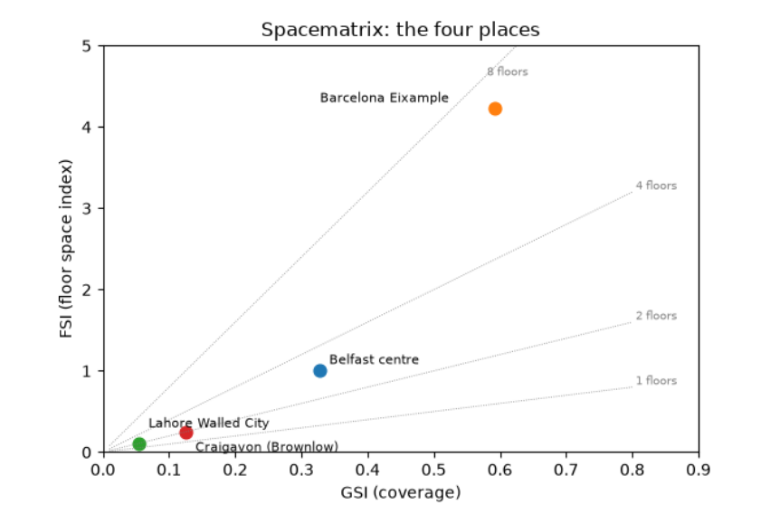
The Spacematrix table and chart place the four areas. The Eixample covers 59 % of its land with buildings (GSI 0.59), at a median footprint of 346 m² (whole blocks of joined apartment buildings) and a floor space index of 4.2: about seven floors on average, with 60 % of buildings carrying a floors tag. Little open ground remains per unit of floor (OSR 0.10). Central Belfast has a third of its land covered, an FSI of 1.0 and about three floors; floors are tagged for a third of buildings, so the rest assume the tagged median of 2. Craigavon is low-rise and open: GSI 0.13, FSI 0.25, under 2 floors. Lahore's figures (GSI 0.05) are an artefact: with most buildings unmapped and almost no floors tagged (1 %), its true coverage is far higher. Always read the 'floors tagged %' and building count before the density.
4.2 Morphometrics: the shape of each building
momepy measures many properties of individual elements. Three useful ones for buildings:
-
Elongation: the ratio of the short to the long side of the smallest rotated rectangle around the footprint (1 = square, near 0 = long and thin, like a terrace row).
-
Circular compactness: footprint area ÷ area of the smallest enclosing circle (1 for a circle, low for L- and courtyard-shaped buildings).
-
Shared walls ratio: the share of the perimeter touching another building. High in terraces and historic cores where buildings are joined; zero for detached houses.
morph = {}
for name, b in blds.items():
    b = b.reset_index(drop=True)
    b = b[b.is_valid & (b.area > 10)].copy()
    b["elongation"] = momepy.elongation(b)
    b["compactness"] = momepy.circular_compactness(b)
    b["shared walls"] = momepy.shared_walls(b) / b.length
    blds[name] = b
    morph[name] = b[["area", "elongation", "compactness", "shared walls"]].median()
    morph[name]["joined to a neighbour %"] = 100 * (b["shared walls"] > 0.05).mean()
morph = pd.DataFrame(morph).T
print(morph.round(2).to_string())

fig, axes = plt.subplots(1, 4, figsize=(14, 4))
for ax, (name, b) in zip(axes, blds.items()):
    b.plot(column="shared walls", ax=ax, cmap="viridis", vmin=0, vmax=0.6, linewidth=0)
    ax.set_title(name, fontsize=10); ax.set_axis_off()
plt.suptitle("Share of each building's perimeter shared with a neighbour (yellow = joined, purple = detached)", fontsize=10)
plt.tight_layout(); plt.show()
area  elongation  compactness  shared walls  joined to a neighbour %
Belfast centre         53.08        0.62         0.54          0.37                    86.55
Barcelona Eixample    346.16        0.47         0.43          0.57                    98.03
Lahore Walled City     89.34        0.65         0.53          0.50                    71.43
Craigavon (Brownlow)  111.09        0.75         0.57          0.00                    29.89
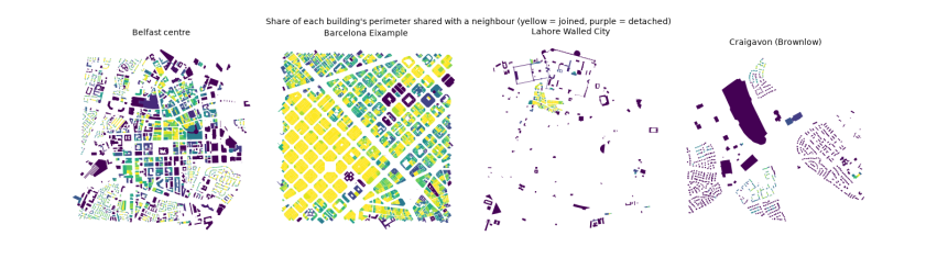
The medians describe a typical building in each place. Barcelona's buildings are large (346 m²) and joined: 98 % share part of their outline with a neighbour, and on average 57 % of a building's perimeter is a party wall. That is the perimeter block: continuous street walls around a courtyard. Belfast's terraces show the same habit at smaller size (53 m², 87 % joined). In Craigavon the median building shares no wall at all, and only 30 % touch a neighbour, mostly semi-detached pairs: detached and semi-detached houses on their own plots. Craigavon's buildings are also the most nearly square (elongation 0.75). The maps show these differences as colour: yellow continuous blocks against purple free-standing houses.