3. Two groups, and a relation
El Niño warms the central Pacific every few years and shifts rainfall around the tropics. Here we test whether it weakens the Indian summer monsoon: first by comparing El Niño years with La Niña years, then by measuring how closely the two series move together.
3.1 Two groups: does El Niño weaken the monsoon?
Thinking it through. What do we want to measure? Whether monsoon rain differs between El Niño and La Niña years, and by how much. What kind of data? Two independent groups of measurements (a year is either one or the other). How do such data behave? Each group mean is uncertain by s/√n; the difference of two means is uncertain by both errors combined, √(s₁²/n₁ + s₂²/n₂). Which test, and why? Welch's t, which does not assume equal spreads; and, as a check that no single extreme year drives the answer, the rank-based Mann–Whitney test. The effect size (Cohen's d) and a confidence interval say how big the difference is, which the p-value alone does not.
Question: is monsoon rainfall in central India lower in El Niño years than in La Niña years? Inputs: for each year 1950–1999, the June–September (JJAS) total of NOAA PSL's Central Indian precipitation index, and the JJAS mean of the Oceanic Niño Index (ONI, °C anomaly of Pacific sea surface temperature). An El Niño year has ONI ≥ +0.5 °C, a La Niña year ≤ −0.5 °C. We express rainfall as a percentage of its mean so the units are easy to read.
oni = read_psl(DATA / "oni.data")
rain = read_psl(DATA / "indiamon.data")
jjas = [6, 7, 8, 9]
m = pd.DataFrame({"oni": oni[jjas].mean(axis=1), "rain": rain[jjas].sum(axis=1, min_count=4)}).dropna()
m["rain_pct"] = 100 * m.rain / m.rain.mean()
m["phase"] = np.where(m.oni >= 0.5, "El Niño", np.where(m.oni <= -0.5, "La Niña", "neutral"))
print(m.groupby("phase").rain_pct.agg(["count", "mean", "std"]).round(1).to_string())
el, la = m.loc[m.phase == "El Niño", "rain_pct"], m.loc[m.phase == "La Niña", "rain_pct"]
count   mean   std
phase
El Niño     10   86.0  13.2
La Niña     11  111.0  12.0
neutral     29  100.7  15.0
Background. In normal years the trade winds blow westward across the tropical Pacific, warm water piles up in the west, and air rises over Indonesia and sinks over the eastern Pacific: the Walker circulation. During El Niño the central and eastern Pacific warm, the rising branch shifts east, and air tends to sink over South Asia, suppressing the clouds and rain of the summer monsoon. La Niña is the opposite phase: a cooler central Pacific, a stronger Walker circulation and, often, a wetter monsoon. So we expect El Niño years to be drier and La Niña years wetter than neutral years. The table above already hints at this: the mean of each group, in % of the 1950–1999 average.
Welch's t-test compares two means without assuming the two groups have equal spread: t = (x̄₁ − x̄₂) / √(s₁²/n₁ + s₂²/n₂), with degrees of freedom from the Welch–Satterthwaite formula. The Mann–Whitney U test asks the same question using only the ranks of the values, so it does not assume normal distributions and is not swayed by one extreme year. Cohen's d is the effect size: the difference in means divided by the pooled standard deviation (about 0.2 small, 0.5 medium, 0.8 large).
welch = stats.ttest_ind(el, la, equal_var=False)
mw = stats.mannwhitneyu(el, la, alternative="two-sided")
sp = np.sqrt(((len(el) - 1) * el.var() + (len(la) - 1) * la.var()) / (len(el) + len(la) - 2))
d = (el.mean() - la.mean()) / sp
print(f"El Niño mean {el.mean():.1f}% (n={len(el)}), La Niña mean {la.mean():.1f}% (n={len(la)}), difference {el.mean() - la.mean():.1f} points")
print(f"Welch t = {welch.statistic:.2f}, df = {welch.df:.1f}, p = {welch.pvalue:.4f}")
print(f"Mann-Whitney U = {mw.statistic:.0f}, p = {mw.pvalue:.4f}")
print(f"Cohen's d = {d:.2f}")
ci = welch.confidence_interval(0.95)
print(f"95% confidence interval for the difference: {ci.low:.1f} to {ci.high:.1f} percentage points")

fig, ax = plt.subplots(figsize=(6.5, 3))
for i, ph in enumerate(["La Niña", "neutral", "El Niño"]):
    v = m.loc[m.phase == ph, "rain_pct"]
    ax.scatter(np.full(len(v), i) + rng.uniform(-0.12, 0.12, len(v)), v, s=18, color=["#1f5c7a", "0.6", "#b91c1c"][i])
    ax.hlines(v.mean(), i - 0.25, i + 0.25, color="k")
ax.set_xticks([0, 1, 2], ["La Niña", "neutral", "El Niño"])
ax.set(ylabel="JJAS rainfall (% of mean)", title="Central India monsoon rainfall by ENSO phase, 1950–1999")
plt.tight_layout(); plt.show()
El Niño mean 86.0% (n=10), La Niña mean 111.0% (n=11), difference -25.0 points
Welch t = -4.53, df = 18.3, p = 0.0003
Mann-Whitney U = 10, p = 0.0017
Cohen's d = -1.99
95% confidence interval for the difference: -36.6 to -13.4 percentage points
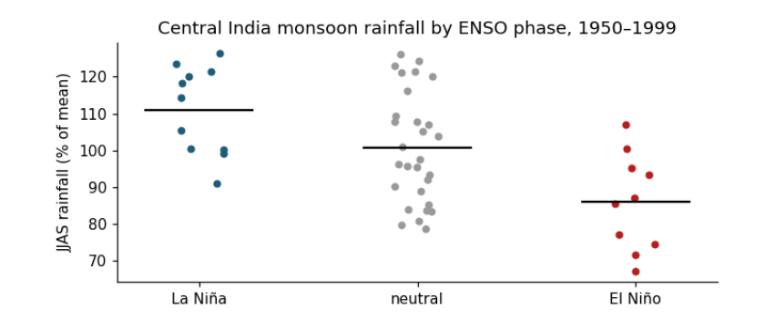
How to read the figure. The x axis has three groups of years, set by the ONI averaged over June–September. The y axis is that year's June–September rainfall as a percentage of the 1950–1999 average, so 100 is a normal monsoon, 90 is 10% below normal. Each dot is one year (spread sideways only so they do not overlap); the black bar is the group's mean. Compare the bars to read the average effect, and the spread of dots to see how reliable it is: if dots of two groups overlap a lot, the effect is weak for any single year even when the means differ.
The comparison above, El Niño against La Niña, mixes two effects. To ask which phase moves the monsoon, and by how much, compare each phase with the neutral years, the "no ENSO" baseline.
neutral = m.loc[m.phase == "neutral", "rain_pct"]
for name, grp in [("El Niño", el), ("La Niña", la)]:
    t_ = stats.ttest_ind(grp, neutral, equal_var=False)
    c_ = t_.confidence_interval(0.95)
    diff = grp.mean() - neutral.mean()
    word = "less" if diff < 0 else "more"
    print(f"{name:8s} vs neutral: {abs(diff):4.1f} percentage points {word} rain (95% CI {c_.low:+.1f} to {c_.high:+.1f}), "
          f"Welch t = {t_.statistic:+.2f}, df = {t_.df:.1f}, p = {t_.pvalue:.3f}")
dry = (el < 90).mean(); dry_n = (neutral < 90).mean()
print(f"share of years with a monsoon more than 10% below normal: El Niño {dry:.0%}, neutral {dry_n:.0%}, La Niña {(la < 90).mean():.0%}")
El Niño  vs neutral: 14.7 percentage points less rain (95% CI -25.3 to -4.2), Welch t = -2.94, df = 17.7, p = 0.009
La Niña  vs neutral: 10.3 percentage points more rain (95% CI +0.8 to +19.7), Welch t = +2.25, df = 22.5, p = 0.034
share of years with a monsoon more than 10% below normal: El Niño 60%, neutral 28%, La Niña 0%
What the results say. Both phases matter, in opposite directions. Read the two lines above as: "in El Niño years, central India received on average about this many percentage points less rain than in neutral years, and we are 95% confident the true difference lies in the bracket". El Niño cut central-India monsoon rain by about 15 percentage points against neutral years (bracket roughly −25 to −4, p ≈ 0.01): a clear effect, though its exact size is uncertain. La Niña added about 10 points (bracket roughly +1 to +20, p ≈ 0.03): an effect in the opposite direction that is smaller and only just distinguishable from zero with 11 years. So El Niño is the stronger and better-supported influence, which is why it dominates forecasts of a weak monsoon. The last line turns the means into risk: a monsoon more than 10% below normal came in about 6 of every 10 El Niño years, about 3 in 10 neutral years, and none of the La Niña years in this period.
What they do not say. Not every El Niño year is dry (some dots sit near 100), so ENSO raises the risk of a weak monsoon rather than deciding it. The sample is 1950–1999 and one regional index; the ENSO–monsoon link is known to weaken and strengthen between decades, and the Indian Ocean Dipole, which also affects the monsoon, is not included.
3.2 Correlation: how strongly do they move together?
Thinking it through. What do we want to measure? How closely Pacific temperature and Indian rain move together, year by year, using all years rather than only the extremes. What kind of data? Pairs of measurements on the same years. How do such data behave? If one drives the other, the points lean along a line; the tighter they hug it, the stronger the link. Which test, and why? Pearson's r for a straight-line link, tested with t = r√(n−2)/√(1−r²); Spearman's ρ (the same on ranks) to check that the answer does not hinge on a straight line or an outlier.
Pearson's r measures linear association, from −1 to +1. To test H₀: r = 0, use t = r√(n − 2)/√(1 − r²) with df = n − 2. Spearman's ρ is Pearson's r computed on ranks, so it captures any steady (monotonic) relation and resists outliers. r² is the share of variance in one variable that a straight line on the other explains.
r, p = stats.pearsonr(m.oni, m.rain_pct)
n = len(m)
t_r = r * np.sqrt(n - 2) / np.sqrt(1 - r ** 2)
rho, p_rho = stats.spearmanr(m.oni, m.rain_pct)
print(f"Pearson r = {r:.2f}, n = {n}, t = {r:.2f} x sqrt({n - 2}) / sqrt(1 - {r:.2f}^2) = {t_r:.2f}, df = {n - 2}, p = {p:.1e}")
print(f"r squared = {r ** 2:.2f}: ONI accounts for {r ** 2:.0%} of the year-to-year variance in this index")
print(f"Spearman rho = {rho:.2f}, p = {p_rho:.1e}")
b = np.polyfit(m.oni, m.rain_pct, 1)
print(f"slope: {b[0]:.1f} percentage points of rainfall per +1 °C of ONI")
resid_sd = np.std(m.rain_pct - np.polyval(b, m.oni), ddof=2)
print(f"a moderate El Niño (ONI +1.0 °C) gives on average {np.polyval(b, 1.0):.0f}% of normal rain; a strong one (+1.5 °C) {np.polyval(b, 1.5):.0f}%;")
print(f"a La Niña (ONI -1.0 °C) {np.polyval(b, -1.0):.0f}%. Single years scatter around the line by about ±{resid_sd:.0f} points (one standard deviation).")

fig, ax = plt.subplots(figsize=(6.5, 3.4))
ax.axvspan(0.5, m.oni.max() + 0.2, color="#b91c1c", alpha=0.08); ax.axvspan(m.oni.min() - 0.2, -0.5, color="#1f5c7a", alpha=0.08)
ax.scatter(m.oni, m.rain_pct, s=18, c=np.where(m.oni >= 0.5, "#b91c1c", np.where(m.oni <= -0.5, "#1f5c7a", "0.55")))
xx = np.linspace(m.oni.min(), m.oni.max(), 10)
ax.plot(xx, np.polyval(b, xx), color="k", lw=1.2, label=f"fitted line: {b[0]:.1f} points per °C")
ax.axhline(100, color="0.6", lw=0.8, ls=":"); ax.axvline(0, color="0.6", lw=0.8, ls=":")
ax.set(xlabel="ONI, June–September mean (°C)", ylabel="JJAS rainfall (% of mean)", title=f"Pacific temperature and central India rain (r = {r:.2f})")
ax.text(0.55, ax.get_ylim()[1] - 3, "El Niño", color="#b91c1c", fontsize=8, va="top"); ax.text(m.oni.min() - 0.15, ax.get_ylim()[1] - 3, "La Niña", color="#1f5c7a", fontsize=8, va="top")
ax.legend(frameon=False, fontsize=8, loc="lower left"); plt.tight_layout(); plt.show()
Pearson r = -0.43, n = 50, t = -0.43 x sqrt(48) / sqrt(1 - -0.43^2) = -3.26, df = 48, p = 2.0e-03
r squared = 0.18: ONI accounts for 18% of the year-to-year variance in this index
Spearman rho = -0.36, p = 1.0e-02
slope: -10.2 percentage points of rainfall per +1 °C of ONI
a moderate El Niño (ONI +1.0 °C) gives on average 90% of normal rain; a strong one (+1.5 °C) 85%;
a La Niña (ONI -1.0 °C) 110%. Single years scatter around the line by about ±15 points (one standard deviation).
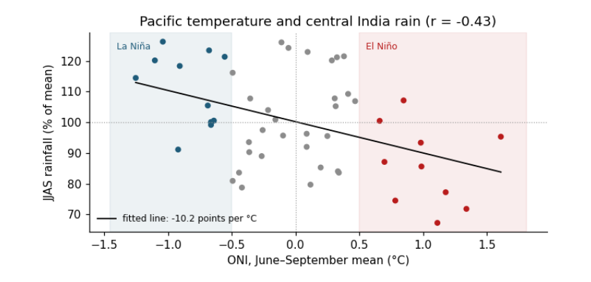
How to read the figure. Each dot is one year. Across: the ONI, how much warmer (right) or cooler (left) than normal the central Pacific was during the monsoon; the red band is El Niño, the blue band La Niña. Up: that year's rainfall, % of normal (the dotted line at 100). The black line is the best straight-line fit; its slope says how many percentage points of rain change per 1 °C of ONI. A cloud of dots that slopes down from left to right means a negative correlation; how tightly the dots hug the line is what r measures.
What the result says. The correlation is negative (warmer central Pacific, drier central India), moderate in size (r ≈ −0.43) and significant (p ≈ 0.002), but ONI explains only about a fifth of the variation (r² ≈ 0.18). The printed lines show why: a moderate El Niño lowers the expected rain by about 10 points, but single years scatter around the line by about ±15 points, so the Pacific shifts the odds without deciding any one monsoon. The two-group comparison above looked stronger because it compared only the extremes, El Niño against La Niña, leaving out the 29 neutral years. Correlation does not by itself show cause; here the physical mechanism (El Niño shifts rising air over the Pacific and suppresses convection over India) is what makes the result meaningful.