1. The ideas behind every test
A hypothesis test answers one narrow question: if nothing special were going on, how surprising would these data be? Every test in this guide, from a coin toss to a flood map, follows the same six steps. Learn them once and every test becomes a variation.
1.1 The six steps
-
State the question in words: is this coin biased? Has June snow cover declined?
-
Write the null hypothesis \(H_0\), the “nothing special” case (the coin is fair; the trend is zero), and the alternative \(H_1\) (the coin is biased; the trend is not zero).
-
Choose a test statistic: one number that summarises how far the data are from what \(H_0\) predicts, such as a \(z\)-score, a \(t\)-value or a \(\chi^2\) value.
-
Find its sampling distribution under \(H_0\): the spread of values the statistic would take if \(H_0\) were true and the data were drawn again and again. Statistical theory gives it for standard tests; a simulation gives it for anything.
-
Compute the p-value: the probability, under \(H_0\), of a statistic at least as extreme as the one observed.
-
Report and interpret: the statistic, its degrees of freedom, the p-value, an effect size and a confidence interval, and what they mean for the question.
1.2 The quantities, and how to read them
| Quantity | What it is and how to read it |
|---|---|
| \(H_0\), \(H_1\) | The null and alternative hypotheses. A test can reject \(H_0\) or fail to reject it; it never proves \(H_0\). |
| \(\alpha\) | The significance level, chosen before looking: the chance of rejecting a true \(H_0\) that you accept. Usually 0.05. |
| p-value | Probability, if \(H_0\) were true, of data at least as extreme as observed. Small means surprising under \(H_0\). It is not the probability that \(H_0\) is true, and not the size of an effect. |
| \(z\) | Distance from a mean in standard deviations, \(z = (x-\mu)/\sigma\). Unitless. $ |
| \(t\) | An estimate divided by its standard error, for example \(t = b/\mathrm{SE}(b)\). Unitless. Read with its degrees of freedom; with few of them, a larger $ |
| \(\chi^2\) | Sum over cells of \((O-E)^2/E\), observed against expected counts. Unitless. Grows with sample size. |
| df | Degrees of freedom: independent pieces of information left after fitting. For a straight line through \(n\) points, \(n-2\). |
| SE | Standard error: how much an estimate would vary between repeated samples. Same units as the estimate. |
| CI | Confidence interval: a range that, in 95% of repeated samples, contains the true value. Same units as the estimate. More informative than a p-value. |
| Effect size | How big the difference or relation is, separately from how certain: Cohen’s \(d\) for means, \(r\) for correlation, Cramér’s \(V\) for tables. |
| Type I error | Rejecting a true \(H_0\) (a false alarm). Its rate is \(\alpha\). |
| Type II error | Failing to reject a false \(H_0\) (a miss). Power is one minus its rate: the chance of detecting a real effect. |
| One- or two-sided | Two-sided asks “different in either direction”; one-sided asks only one direction and must be chosen before seeing the data. |
1.3 Assumptions: where tests go wrong
Every test assumes something about the data, and climate data break one assumption more often than any other: independence. Today’s temperature resembles yesterday’s; one flooded field implies the next. Treated as independent, such data look far more informative than they are, and p-values come out too small. The guide shows the effect and two simple remedies: counting the effective number of independent years for a trend, and thinning a map before testing it. The other common assumptions are approximate normality (for \(z\) and \(t\)), equal spread in two groups (dropped by Welch’s test) and large enough expected counts (for \(\chi^2\), at least about five per cell). Rank-based tests (Mann–Whitney, Spearman, Mann–Kendall) drop normality.
1.4 Setup
This notebook runs every test in the guide on real data. Short examples come first, to build intuition with numbers small enough to check by hand; then each test is applied to a real question from climate, El Niño and the monsoon, snow cover, and radar flood mapping. Every printed number is explained: what goes in, what comes out, its units, and how to read it.
Libraries: numpy (arithmetic on arrays), pandas (tables), scipy.stats (the tests themselves) and matplotlib (figures). A fixed random seed makes the simulations repeat exactly.
import urllib.request
from pathlib import Path

import numpy as np
import pandas as pd
import matplotlib.pyplot as plt
from scipy import stats

rng = np.random.default_rng(42)
plt.rcParams.update({"figure.dpi": 110, "axes.spines.top": False, "axes.spines.right": False})
DATA = Path("data"); DATA.mkdir(exist_ok=True)
SOURCES = {
    "hadcrut5.csv": "https://www.metoffice.gov.uk/hadobs/hadcrut5/data/HadCRUT.5.0.2.0/analysis/diagnostics/"
                    "HadCRUT.5.0.2.0.analysis.summary_series.global.annual.csv",
    "oni.data": "https://psl.noaa.gov/data/correlation/oni.data",
    "indiamon.data": "https://psl.noaa.gov/data/correlation/indiamon.data",
    "nh_snow.txt": "https://climate.rutgers.edu/snowcover/files/moncov.nhland.txt",
    # a small table made for this guide from the radar manual's Sentinel-1 export (see data_local/SOURCE.txt)
    "sindh_sar_1km.csv": "https://raw.githubusercontent.com/AhmadAmmar/AhmadAmmar.github.io/main/guides/hypothesis-testing/notebooks/data_local/sindh_sar_1km.csv",
}
LOCAL = Path("data_local")                  # present when the notebook runs inside the guide's own folder
for name, url in SOURCES.items():
    if not (DATA / name).exists() and (LOCAL / name).exists():
        (DATA / name).write_bytes((LOCAL / name).read_bytes())
    if not (DATA / name).exists():
        req = urllib.request.Request(url, headers={"User-Agent": "hypothesis-notebook/1.0"})
        (DATA / name).write_bytes(urllib.request.urlopen(req, timeout=120).read())
    print(f"{name:14s} {(DATA / name).stat().st_size / 1e3:8.1f} kB")


def read_psl(path):
    """NOAA PSL index files: one row per year, twelve monthly values; -99.9 and -999.9 mean missing."""
    rows = []
    for line in Path(path).read_text().splitlines():
        parts = line.split()
        if len(parts) == 13 and parts[0].isdigit():
            rows.append([int(parts[0])] + [float(v) for v in parts[1:]])
    t = pd.DataFrame(rows, columns=["year", *range(1, 13)]).set_index("year")
    return t.mask(t <= -99)
hadcrut5.csv        7.0 kB
oni.data            6.7 kB
indiamon.data       3.5 kB
nh_snow.txt        13.3 kB
sindh_sar_1km.csv    755.1 kB
1.5 A coin and a p-value
Thinking it through. What do we want to measure? Whether a coin favours heads. What kind of data? A count of successes out of a fixed number of independent tries. How do such data behave? With a fair coin the count follows the binomial distribution, centred on n/2 with a spread of √(n × 0.5 × 0.5) = 5 heads for 100 tosses. Which test, and why? The exact binomial test, because we know that distribution exactly; the z-test is its normal approximation, fine for large n. The chapter Calculating by hand works a 10-toss version line by line.
Every hypothesis test has the same shape. A null hypothesis (H₀) says "nothing special is going on". A test statistic summarises the data in one number. Under H₀ that number has a known spread of values, its sampling distribution. The p-value is the probability, if H₀ were true, of a statistic at least as extreme as the one observed. A small p means the data would be surprising if H₀ were true.
Short example: a coin gives 60 heads in 100 flips. H₀: the coin is fair, P(heads) = 0.5. Statistic: the number of heads. We find the p-value three ways: by simulating 100,000 fair coins, exactly from the binomial distribution, and with the normal approximation (a z-score).
heads, n = 60, 100
sims = rng.binomial(n, 0.5, size=100_000)
p_sim = np.mean(np.abs(sims - 50) >= abs(heads - 50))            # two-sided: as far from 50 in either direction
p_exact = stats.binomtest(heads, n, 0.5).pvalue
z = (heads - n * 0.5) / np.sqrt(n * 0.5 * 0.5)                  # (observed - expected) / standard deviation
p_z = 2 * stats.norm.sf(abs(z))
z_cc = (abs(heads - n * 0.5) - 0.5) / np.sqrt(n * 0.5 * 0.5)     # continuity correction: counts are whole numbers
p_cc = 2 * stats.norm.sf(z_cc)
print(f"simulation p = {p_sim:.4f}   exact binomial p = {p_exact:.4f}")
print(f"normal approximation: z = {z:.2f}, p = {p_z:.4f};  with continuity correction z = {z_cc:.2f}, p = {p_cc:.4f}")

fig, ax = plt.subplots(figsize=(7, 2.8))
ax.hist(sims, bins=np.arange(30, 71) - 0.5, color="#cbd5e1")
ax.hist(sims[np.abs(sims - 50) >= 10], bins=np.arange(30, 71) - 0.5, color="#b91c1c", label="as extreme as 60 or more")
ax.axvline(60, color="k", lw=1)
ax.set(xlabel="heads in 100 flips of a fair coin", ylabel="simulations", title="The sampling distribution under H₀")
ax.legend(frameon=False, fontsize=8); plt.tight_layout(); plt.show()
simulation p = 0.0571   exact binomial p = 0.0569
normal approximation: z = 2.00, p = 0.0455;  with continuity correction z = 1.90, p = 0.0574
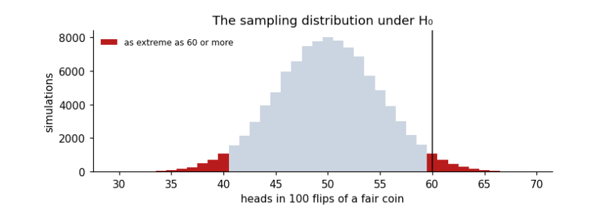
Reading it: the grey histogram is what a fair coin produces; the red tails are results at least as far from 50 as 60 is. Their share, about 0.057, is the p-value. With the usual threshold α = 0.05, 0.057 is just above it, so we would not reject H₀: 60 heads is a little unusual but not convincing evidence of a biased coin. The simulation and the exact binomial agree. The plain normal approximation gives 0.046, which would wrongly fall below 0.05: it treats the count of heads as continuous, while it can only be a whole number. The continuity correction subtracts half a count from the distance to the expected value, and brings the approximation back to 0.057. Approximations are convenient; when an exact test is available, use it, especially with small counts.
Two warnings that apply to every test below. A p-value is not the probability that H₀ is true, and a large p-value does not show H₀ is true; it only says the data are not surprising under H₀. And a tiny p-value says nothing about how big or important an effect is: for that we need an effect size and a confidence interval.