2. One value, and a trend
Two of the most common questions asked of climate data are whether a single value is unusual, and whether a series has a trend. The \(z\)-test answers the first when the spread is known. The \(t\)-test answers the second, and its degrees of freedom show why a trend from few, or dependent, years deserves caution.
2.1 The z-test: is one value unusual?
Thinking it through. What do we want to measure? How unusual one value is against a reference. What kind of data? One new measurement, and a reference set whose mean and spread we treat as known. How do such data behave? Measurements of a stable quantity scatter around their mean, often close to a normal (bell-shaped) curve, so the distance from the mean in units of standard deviation says how rare a value is. Which test, and why? The z-score, because the spread is taken as known; if it had to be estimated from a few values, t would replace z.
The z-score measures how many standard deviations (σ) a value lies from a mean (μ): z = (x − μ) / σ. If values are normally distributed, about 95% fall within z = ±1.96, and the two-sided p-value is 2 × P(Z > z).
Short example, by hand: a class has a mean exam mark of 60 with σ = 10. A mark of 78 gives z = (78 − 60)/10 = 1.8, and p = 2 × 0.036 = 0.072.
Real example: how unusual was 2024's global temperature compared with the climate of 1961–1990?
g = pd.read_csv(DATA / "hadcrut5.csv").rename(columns={"Time": "year", "Anomaly (deg C)": "anom"})[["year", "anom"]]
g = g[g.year <= 2024]
base = g[g.year.between(1961, 1990)].anom
mu, sigma = base.mean(), base.std(ddof=1)
x = g.loc[g.year == 2024, "anom"].iloc[0]
z = (x - mu) / sigma
print(f"1961-1990: mean μ = {mu:.3f} °C, standard deviation σ = {sigma:.3f} °C (n = {len(base)})")
print(f"2024: x = {x:.3f} °C  ->  z = ({x:.3f} - {mu:.3f}) / {sigma:.3f} = {z:.1f}")
print(f"two-sided p = {2 * stats.norm.sf(abs(z)):.1e}")
print(f"by hand, the class example: z = 1.8, p = {2 * stats.norm.sf(1.8):.3f}")

fig, ax = plt.subplots(figsize=(7, 2.8))
xs = np.linspace(mu - 4 * sigma, x + 0.1, 400)
ax.plot(xs, stats.norm.pdf(xs, mu, sigma), color="#1f5c7a", label="normal curve from 1961–1990 (μ, σ)")
ax.hist(base, bins=8, density=True, color="#cbd5e1", label="the 30 years 1961–1990")
for k in (1, 2, 3):
    ax.axvline(mu + k * sigma, color="0.75", lw=0.8, ls=":")
ax.axvline(x, color="#b91c1c", lw=2, label=f"2024: {x:.2f} °C (z = {z:.1f})")
ax.set(xlabel="Global temperature anomaly (°C, vs 1961–1990)", ylabel="probability density", title="How far 2024 lies from the 1961–1990 climate")
ax.legend(frameon=False, fontsize=8, loc="upper center"); plt.tight_layout(); plt.show()
1961-1990: mean μ = 0.008 °C, standard deviation σ = 0.170 °C (n = 30)
2024: x = 1.181 °C  ->  z = (1.181 - 0.008) / 0.170 = 6.9
two-sided p = 5.5e-12
by hand, the class example: z = 1.8, p = 0.072
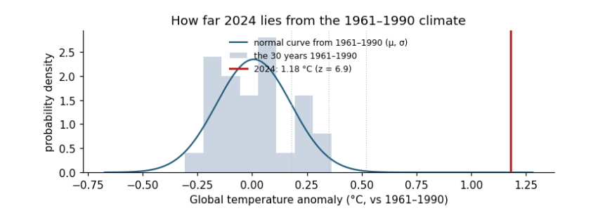
How to read the figure. The x axis is the temperature anomaly in °C. The grey bars are the 30 years of the reference period, piled up by value; the blue curve is the normal distribution with the same mean μ and standard deviation σ. The dotted lines mark μ + 1σ, 2σ and 3σ: about 68%, 95% and 99.7% of a normal distribution lies within them. The red line is 2024. The p-value is the area under the blue curve beyond the red line (on both sides for a two-sided test): it is so small that it cannot be seen.
What the result says. 2024 lies about 7 standard deviations above the 1961–1990 mean, and the p-value is about 5 × 10⁻¹². Under the climate of 1961–1990, a year this warm would essentially never happen: the climate itself has changed. What it does not say. The z-test does not say why; for that we need the trend test and the physics. Units: z has none (it is a count of σ); μ, σ and x are in °C. Caveat: the z-test assumes the reference years are independent draws from a normal distribution with a stable mean; here the 1961–1990 years already contain a little trend, which makes σ slightly larger and the test slightly conservative.
2.2 The t-test for a trend
Thinking it through. What do we want to measure? Whether a quantity changes steadily over time, and how fast. What kind of data? Pairs (year, value). How do such data behave? Each value is trend plus noise; the fitted slope would come out a little different with different noise, and that wobble is its standard error, estimated from the scatter around the line. Which test, and why? t = slope / SE with n − 2 degrees of freedom: t rather than z because the scatter is estimated from the same data, and n − 2 because the line used up two numbers. Neighbouring years are alike (autocorrelation), so we also shrink n to the effective number of independent years.
A trend's slope b is estimated from data, so it has a standard error SE(b). The t-statistic is t = b / SE(b): how many standard errors the slope is from zero. Under H₀ (no trend) it follows a t distribution with degrees of freedom df = n − 2 (n points, minus the two numbers fitted: slope and intercept). Degrees of freedom count the independent pieces of information left after fitting; fewer means wider tails and larger p-values.
Short example, by hand: five years with slope b = 0.02 °C/yr and SE = 0.008 give t = 2.5, df = 3, and p = 0.088: with so few points, even t = 2.5 is not strong evidence.
print(f"by hand: t = 0.02 / 0.008 = 2.5, df = 3, two-sided p = {2 * stats.t.sf(2.5, 3):.3f}")
w = g[g.year.between(1983, 2024)]
fit = stats.linregress(w.year, w.anom)
t_naive = fit.slope / fit.stderr
resid = w.anom - (fit.intercept + fit.slope * w.year)
r1 = np.corrcoef(resid[:-1], resid[1:])[0, 1]
n = len(w); n_eff = n * (1 - r1) / (1 + r1)
se_eff = fit.stderr * np.sqrt((n - 2) / (n_eff - 2))
t_eff = fit.slope / se_eff
print(f"global 1983-2024: b = {fit.slope * 10:.3f} °C/decade, SE = {fit.stderr * 10:.3f}, t = {t_naive:.1f}, df = {n - 2}, p = {fit.pvalue:.1e}")
print(f"lag-1 autocorrelation r1 = {r1:.2f} -> effective n = {n_eff:.1f}; corrected SE = {se_eff * 10:.3f}, t = {t_eff:.1f}, "
      f"df = {n_eff - 2:.1f}, p = {2 * stats.t.sf(t_eff, n_eff - 2):.1e}")
ci = fit.slope * 10 + np.array([-1, 1]) * stats.t.ppf(0.975, n_eff - 2) * se_eff * 10
print(f"95% confidence interval for the trend: {ci[0]:.3f} to {ci[1]:.3f} °C per decade")

fig, ax = plt.subplots(figsize=(7, 2.8))
ax.plot(w.year, w.anom, "o", ms=3, color="0.4", label="each year")
yr = w.year.to_numpy(float); mid = yr.mean(); line = fit.intercept + fit.slope * yr
ax.plot(yr, line, color="#b91c1c", label=f"trend {fit.slope * 10:.2f} °C per decade")
for lo in (ci[0], ci[1]):
    ax.plot(yr, fit.intercept + fit.slope * mid + lo / 10 * (yr - mid), color="#b91c1c", lw=0.8, ls="--")
ax.set(xlabel="Year", ylabel="Anomaly (°C)", title="Global temperature 1983–2024 with its trend and 95% range of slopes")
ax.legend(frameon=False, fontsize=8); plt.tight_layout(); plt.show()
by hand: t = 0.02 / 0.008 = 2.5, df = 3, two-sided p = 0.088
global 1983-2024: b = 0.216 °C/decade, SE = 0.013, t = 16.8, df = 40, p = 1.1e-19
lag-1 autocorrelation r1 = 0.22 -> effective n = 27.0; corrected SE = 0.016, t = 13.3, df = 25.0, p = 8.0e-13
95% confidence interval for the trend: 0.182 to 0.249 °C per decade
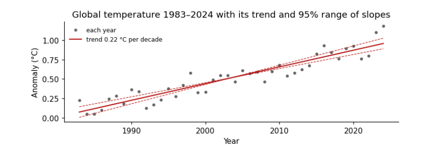
How to read the figure. Each grey dot is one year (x: the year; y: its anomaly in °C). The red line is the fitted trend; its steepness is the slope b. The dashed lines are the steepest and shallowest slopes inside the 95% confidence interval, pivoting on the middle year: the true trend is very likely somewhere between them. The scatter of dots around the line is the year-to-year noise (El Niño, volcanoes, weather) that makes the slope uncertain.
What the result says. The slope is about 0.22 °C per decade; t is about 17 (13 after allowing for autocorrelation) and p is tiny, so a zero trend is ruled out. The confidence interval is the more useful output: we are 95% confident the true trend lies between about 0.18 and 0.25 °C per decade. Allowing for autocorrelation (neighbouring years are alike, r₁ ≈ 0.2) reduces the 42 years to about 27 independent ones and widens the interval, but here it changes nothing important. With weaker trends or stronger autocorrelation it can turn a "significant" result into an insignificant one.