The whole guide on one page
1. The science behind the images
1.1 Why radar sees what it sees
A radar sends a pulse and times its return. Distance comes from time, as \(R = ct/2\), where \(c\) is the speed of light and the 2 accounts for the trip out and back. Sentinel-1 uses C band: a frequency of 5.405 GHz, which is a wavelength of \(\lambda = c/f \approx 5.5\) cm. Features much smaller than this look smooth to the radar, which is why calm water and tarmac act like mirrors.
The sensor looks sideways, not straight down. If it looked straight down, two points at equal distance either side would return together and could not be told apart. Looking sideways at about 29 to 46 degrees in this mode solves that, and also causes the distortions described below.
1.2 What backscatter is
The radar equation says how much power returns:
Here \(P_t\) is power sent, \(G\) antenna gain, \(R\) range and \(\sigma\) the radar cross-section of the target. Everything but \(\sigma\) is known about the instrument and geometry, so it can be removed by calibration. For a surface, \(\sigma\) is divided by the ground area to give \(\sigma^0\) (sigma nought), a dimensionless ratio that can be compared between places and dates.
1.3 What a decibel is
Backscatter spans many orders of magnitude, from about 0.001 for calm water to above 10 for a building’s corner. A logarithmic scale fits this on a readable range:
| Linear | dB | Meaning |
|---|---|---|
| 0.001 | \(-30\) | A thousandth of the reference |
| 0.01 | \(-20\) | A hundredth |
| 0.1 | \(-10\) | A tenth |
| 1 | 0 | Equal to the reference |
| 2 | \(+3\) | About double |
| 10 | \(+10\) | Ten times |
Decibels are ratios, so a difference in dB is a ratio in power. A change from \(-10\) to \(-13\) dB means half the power returned, wherever it happens on the scale. Negative values are normal and do not mean negative energy: they mean less than the reference.
# Why averaging in dB is wrong.
Take two pixels at \(-30\) and \(0\) dB. Their mean in dB is \(-15\) dB. In linear units, the mean of 0.001 and 1 is 0.5005, which is \(-3\) dB. The dB mean is lower by 12 dB, a factor of about 16 in power, because a logarithm gives the dim pixel too much weight. So we average in linear power, as mean_db() does in Chapter 2. Over a year of London scenes this matters most at strong targets, whose returns vary.
1.4 Polarisation: what VV and VH tell us
The radar’s wave oscillates in one plane. Sentinel-1 sends vertically (V) and receives both V and horizontal (H). Each surface changes this differently:
| Mechanism | What happens and where |
|---|---|
| Surface scattering | Rough ground reflects some energy back, mostly keeping polarisation, so VV is above VH |
| Volume scattering | Repeated scattering among leaves and branches scrambles polarisation, so VH rises |
| Double bounce | Ground and wall form a corner that returns energy strongly, so VV is very high, as in cities and flooded forest |
| Specular reflection | A smooth surface reflects energy away, so both are low, as on calm water |
The ratio VV minus VH (in dB, which is a ratio in linear terms) separates these partly, which is why it serves as the third band in our colour image.
1.5 Speckle
# What it is.
A pixel holds many scatterers. Their returns add as waves with random phases, sometimes reinforcing and sometimes cancelling. So uniform ground looks grainy, even with a perfect instrument. Viewed the same way, the same ground gives the same grain, which makes it a form of interference and not random instrument noise.
# The model.
Speckle is multiplicative: observed intensity \(I\) is the true backscatter \(\sigma^0\) times a random factor \(n\) with mean 1:
Multiplicative means brighter areas have larger swings in linear units, and a logarithm turns these into a roughly constant spread. \(L\) is the number of looks, or independent samples averaged. It can be estimated from a uniform area as the equivalent number of looks:
# Measured here.
Over the most uniform 300 m patch near central London, ENL is 4.4 in one scene and 20.9 in the mean of 149 scenes. The increase is less than 149-fold, because the patch is not perfectly uniform and because real changes through the year remain. This also suggests a limit: averaging removes speckle at the cost of time detail, and filters such as Lee or Refined Lee remove it at the cost of spatial detail.
1.6 What has been done to the data
The Earth Engine collection COPERNICUS/S1_GRD holds Ground Range Detected scenes, already processed as follows:
-
Orbit file: precise position of the satellite.
-
GRD border noise removal: low-value strips at scene edges.
-
Thermal noise removal: the instrument’s own noise.
-
Radiometric calibration: digital numbers to \(\sigma^0\).
-
Terrain correction: moved to map position with a digital elevation model.
-
Conversion to dB.
It has not had speckle filtering or radiometric terrain flattening, so slopes facing the satellite stay bright. “Detected” also means phase has been discarded, so these scenes cannot be used for interferometry; heights and motion need the single look complex (SLC) product, or ready-made interferograms such as ASF HyP3 for Sentinel-1 and NISAR’s GUNW.
1.7 Three distortions of mountains
Because radar measures distance, tall things shift towards the sensor:
-
Foreshortening: slopes facing the radar look compressed and bright.
-
Layover: the top of a steep slope or tower returns before its base, and appears displaced towards the sensor.
-
Shadow: slopes facing away receive no signal and look black.
You can see the first of these in the hills in the lower left of the Sindh map, and the second in London’s towers. In both cases brightness reflects geometry, not material. In high mountains these are not details: along the Karakoram Highway large parts of every valley are in layover or shadow from one pass direction, which is why ascending and descending passes are combined and why such pixels are masked before any height or motion is read from them.
1.8 Wavelength: C band and L band
The wavelength decides what the radar interacts with. Sentinel-1’s C band (\(\lambda \approx 5.5\) cm) is scattered by leaves, twigs and small stones, so it sees the top of a canopy and the texture of a surface. NISAR’s L band (\(\lambda \approx 24\) cm, launched 2025) passes through leaves and is scattered by trunks, branches and the ground, so it sees deeper into vegetation. For interferometry this matters most: longer waves change less when leaves move or snow settles, so L-band images taken twelve days apart still match on slopes where C-band images have lost all phase coherence. In steep, vegetated, debris-covered mountains such as the Karakoram this is the difference between a usable measurement and noise.
1.9 Phase: what interferometry measures
Every radar pixel is a complex number: an amplitude (the backscatter used so far) and a phase, the fraction of a wavelength left over on the trip to the ground and back. One image’s phase looks random, because each pixel holds many scatterers. But two images of the same place taken from nearly the same orbit share that randomness, so multiplying one by the complex conjugate of the other cancels it and leaves the phase difference, the interferogram. That difference is a sum of contributions (Hanssen 2001):
Only the first three carry signal. The flat-earth term is a ramp from the curvature of the reference ellipsoid and is removed with the orbits. Which of the other two is wanted decides the job:
- Heights (a DEM). Choose a pair a few days apart, so the ground has not moved, with a large perpendicular baseline \(B_\perp\) (distance between the two orbits). The topographic phase gives height,
where \(R_0\) is slant range, \(\theta\) the look angle, and \(h_a\) the height of ambiguity: the height change that makes one full fringe. A larger baseline gives a smaller \(h_a\), finer height and denser fringes.
- Motion. Remove the topography with an existing DEM; what remains is motion along the line of sight,
There is no baseline in this equation: one fringe is half a wavelength of motion, 2.8 cm for Sentinel-1 and 12 cm for NISAR. That is why interferometry sees millimetres, and also why any DEM error or atmospheric delay leaks straight into apparent motion.
1.10 Unwrapping
The interferometer measures phase only modulo \(2\pi\): the true phase is the measured value plus an unknown whole number of cycles, which is why interferograms look like repeating rainbow fringes. Unwrapping recovers the missing cycles and turns the fringes into one continuous surface. The usual tool is SNAPHU (Chen and Zebker 2001), which finds the solution of lowest statistical cost over the whole image. Practical settings, which decide whether it works at all (Shah 2026b): use as few tiles as memory allows, because every seam between tiles is a place the solution can break; give tiles an overlap of 100 to 200 pixels (an overlap of zero leaves nothing to align and often gives an empty output); start with the minimum cost flow (MCF) method rather than a spanning tree; and set the cost mode to TOPO for heights and DEFO for motion. Unwrapping fails where coherence is low (water, snow, layover, fast change), so those pixels are masked, not guessed.
1.11 Polarimetry and covariance
A dual-polarised image gives two intensities, VV and VH (or HH and HV). A fully polarimetric radar also keeps the phase between polarisations, and the natural way to store that is a covariance matrix per pixel. NISAR’s geocoded covariance product (GCOV) does this (Shiroma et al. 2024): its diagonal terms (HHHH, HVHV, VVVV, VHVH) are the familiar powers, converted to decibels with \(10\log_{10}\), and are already terrain corrected (\(\gamma^0\)); the off-diagonal terms, when present, are complex and allow decompositions into surface, double-bounce and volume scattering (Freeman–Durden) or entropy, anisotropy and angle (Cloude–Pottier). One file can hold two frequency groups with different polarisations, and each comes with a mask: values 1 to 5 are valid (the sub-swath the data came from), 0 is invalid and 255 is outside the image. The gaps the mask leaves are a statement about quality and should be respected, not filled (Shah 2026a).
1.12 Reading rules
-
Dark usually means smooth, or facing away. It does not always mean water.
-
Bright usually means rough, wet, or a corner. It does not always mean buildings.
-
Compare like with like: the same pass direction and season.
-
Average in linear power, and report in dB.
-
Trust change between dates more than a single absolute value.
2. How to read a radar image: London
2.1 What the satellite measures
Sentinel-1 sends microwave pulses at a wavelength of about 5.5 cm and records what returns. It supplies its own signal, so it works at night and sees through cloud. The picture therefore shows how surfaces send energy back, which is different from colour. Three things control the return: how rough a surface is at the scale of the wavelength, its geometry, and how wet it is.
| Surface | Why it looks as it does |
|---|---|
| Calm water | A smooth mirror reflects the pulse away, so it looks dark |
| Vegetation | Leaves and branches scatter in many directions, so it looks moderate, with strong VH |
| Buildings | Walls and ground form corners that send the pulse straight back, so they look very bright |
2.2 The numbers
The image holds backscatter, \(\sigma^0\), usually in decibels:
So 10 dB more is ten times the power, and 3 dB is about double. Polarisation is written as sent and received: VV goes out and returns vertically, whereas VH goes out vertically and returns horizontally. Volume scattering in vegetation changes polarisation, so VH responds strongly to it.
2.3 Step 1: choose the scenes
We take all ascending Interferometric Wide scenes over London in 2024: 149 of them. Keeping one pass direction matters, because a building looks different from each side. From the code: src/sarlib.py, s1(), lines 17--23
def s1(region, start, end, orbit=None):
    """Sentinel-1 ground range scenes in dual polarisation; values are already calibrated backscatter in dB."""
    c = (ee.ImageCollection("COPERNICUS/S1_GRD").filterBounds(region).filterDate(start, end)
         .filter(ee.Filter.eq("instrumentMode", "IW"))
         .filter(ee.Filter.listContains("transmitterReceiverPolarisation", "VV"))
         .filter(ee.Filter.listContains("transmitterReceiverPolarisation", "VH")))
    return c.filter(ee.Filter.eq("orbitProperties_pass", orbit)) if orbit else c
2.4 Step 2: average in the right units
Decibels are logarithms, so averaging them understates bright targets. We convert to linear power, average, and convert back: From the code: src/sarlib.py, mean_db(), lines 30--32
def mean_db(collection, band):
    """Average in linear power and return to dB, because averaging decibels understates bright targets."""
    return collection.select(band).map(to_linear).mean().log10().multiply(10).rename(band)
2.5 Step 3: see why averaging is needed
Radar images have a grain called speckle, which arises when returns from many small scatterers within a pixel interfere. It is not noise in the usual sense, since it would repeat exactly from an identical view, but it hides detail. Over the most uniform 300 m patch in this view, chosen by the code, the spread of VV falls from 2.05 dB in one scene (2024-01-07) to 0.78 dB in the mean of the year (Figure 2.1).
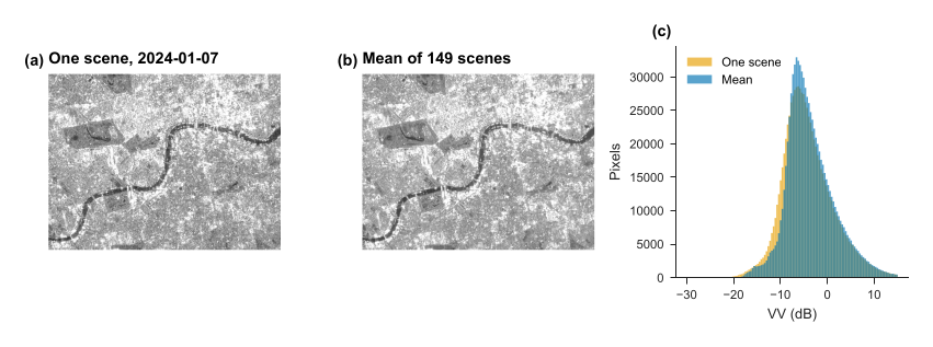
Figure 2.1. Central London: one scene (a), the mean of the year (b), and the distribution of values (c).
2.6 Step 4: build a false-colour image
No single band shows everything (Figure 2.2), so we put three in the display channels: VV as red, VH as green, and VV minus VH as blue.
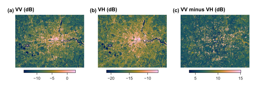
Figure 2.2. The three bands, each stretched between its 2nd and 98th percentiles.
2.7 Reading the map
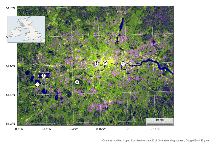
Figure 2.3. London in radar, 2024. VV as red, VH as green, VV minus VH as blue. Numbers are explained in Table 2.1. British National Grid.
| Place | VV (dB) | VH (dB) | VV minus VH |
|---|---|---|---|
| Heathrow Airport | 5.7 | -0.7 | 6.4 |
| River Thames, central London | -14.8 | -20.5 | 5.8 |
| Hyde Park | -8.1 | -14.2 | 6.2 |
| Canary Wharf | 8.8 | 1.9 | 6.9 |
| Richmond Park | -12.8 | -19.1 | 6.3 |
| Reservoir south-west of Heathrow | -17.8 | -26.7 | 8.9 |
Table 2.1. Measured values, averaged over a small circle at each numbered place in Figure 2.3.
Look at the map in this order:
-
Water (2, 6). The Thames and the reservoirs are the darkest features. The river’s width changes on the map partly because a narrow channel can be mixed in one pixel with its bright banks and bridges.
-
The dense centre (4). Canary Wharf is extremely bright, because towers form strong corners. Its value is one of the highest in the table.
-
Green space (3, 5). Hyde Park and Richmond Park stand out as dark green holes in the city. Both polarisations are low, since grass is fairly smooth at this wavelength.
-
Airport (1). Heathrow’s runways are dark stripes, smooth like water, surrounded by bright buildings.
A caution: the mean at a marked place depends on exactly where the circle falls, and at the river it can include bridge and bank returns.
3. Mapping a flood: Sindh, 2022
3.1 The question
In 2022 severe floods covered large parts of Pakistan. Cloud often blocks optical satellites during such events, while radar keeps seeing. Open floodwater is smooth, so it turns dark. We therefore look for land that was not dark in a normal year and turned dark during the flood. The area here runs from Manchar Lake along the Indus.
3.2 Step 1: a before and an after
We take the mean VV over the same weeks of two years, 25 August to 15 September in 2021 (12 scenes) and 2022 (12 scenes), so the season is alike. VV is the usual choice for open water, because it separates smooth water well from rougher land.
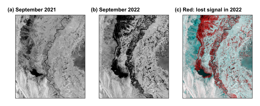
Figure 3.1. September 2021 (a), September 2022 (b), and a colour combination (c) in which a surface that lost signal in 2022 appears red. UTM 42N.
3.3 Step 2: choose a threshold from the data
Water and land form two groups in the histogram, so we need the value that best separates them. Otsu’s method tries every value \(t\), and keeps the one that maximises the variance between the two groups:
where \(w\) is the share of pixels in each group and \(\mu\) its mean. Here it gives -14.1 dB (Figure 3.2). From the code: src/sarlib.py, otsu(), lines 61--69
def otsu(values, bins=256):
    """The threshold that best separates two groups: it maximises the variance between them (Otsu, 1979)."""
    v = values[np.isfinite(values)]
    count, edges = np.histogram(v, bins=bins)
    mids = (edges[:-1] + edges[1:]) / 2
    w = np.cumsum(count).astype(float)
    m = np.cumsum(count * mids)
    between = (m[-1] * w / w[-1] - m) ** 2 / (w * (w[-1] - w) + 1e-9) * w[-1]
    return float(mids[np.argmax(between)])
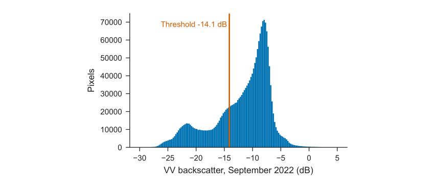
Figure 3.2. Backscatter in 2022, with the threshold.
3.4 Step 3: separate flood from usual water
Three rules define flood: below the threshold in 2022, above it in 2021, and water less than 50% of the time in the JRC Global Surface Water record. From the code: src/02_sindh_flood.py, lines 25--28
thr = otsu(after)
wet_after, wet_before = after < thr, before < thr
flood = wet_after & ~wet_before & (occ < 50)
permanent = wet_after & (occ >= 50)
3.5 Reading the map
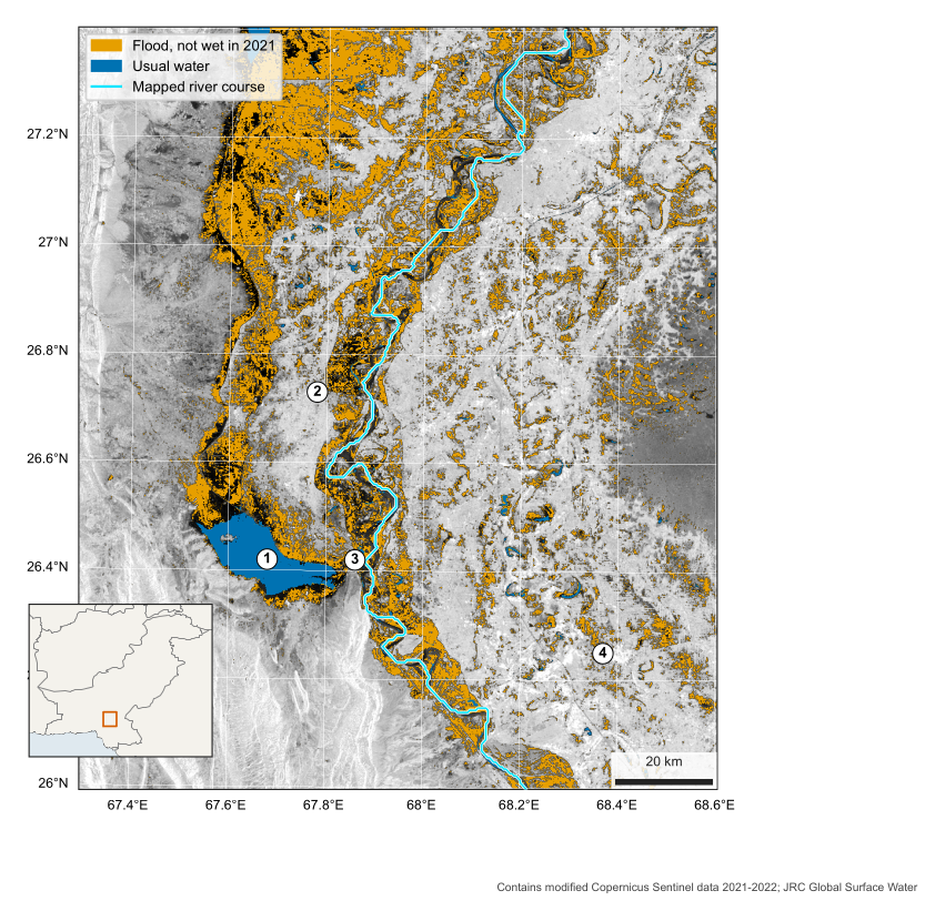
Figure 3.3. Water in Sindh, September 2022, over VV backscatter. 1 Manchar Lake, 2 Dadu, 3 Sehwan, 4 Nawabshah. UTM 42N.
| What to look for | How to read it |
|---|---|
| Around Manchar Lake (1) | The usual lake is blue. The orange beyond it is new water spread along the foot of the western hills |
| Along the Indus | A wide orange band follows the river, with the usual channel in blue within it |
| Round Dadu (2) | Bright, higher ground stands out between flooded land, so settlement is a visible island |
| Round Sehwan (3) | Hills pinch the valley here, and the flood narrows |
| West, lower left | Bright ridges facing the satellite are the hills. They are terrain, not buildings |
3.6 Results
The map shows about 3,458 km\(^2\) of flood within the 20,415 km\(^2\) scene, and 348 km\(^2\) of usual water. Moving the threshold by 2 dB either way gives 3,145 and 3,345 km\(^2\), so the choice matters less than the limits below.
3.7 What this cannot tell you
-
Not validated. This is a teaching estimate, and it has not been compared with optical images or field reports.
-
Rice and wet soil. Flooded fields and irrigated land in September can look like flood. This is likely in scattered patches, especially in the east.
-
Hidden water. Water beneath trees or crops, or among buildings, may be missed because those surfaces stay bright.
-
Three weeks in one image. A mean covers several passes, so it shows water present for much of the period, and not one moment.
-
Black areas. Dark in both years, these may be standing water or smooth sand. They are not counted as flood.
References
Chen, Curtis W., and Howard A. Zebker. 2001. “Two-Dimensional Phase Unwrapping with Use of Statistical Models for Cost Functions in Nonlinear Optimization.” Journal of the Optical Society of America A 18 (2): 338–51.
Hanssen, Ramon F. 2001. Radar Interferometry: Data Interpretation and Error Analysis. Kluwer Academic.
Shah, Muddasir. 2026a. From VV/VH in dB to Covariance Matrices: First Lessons from NISAR L2 GCOV over the Indus Delta Mangroves. LinkedIn article, 27 April. https://www.linkedin.com/pulse/from-vvvh-db-covariance-matrices-first-lessons-nisar-l2-muddasir-shah-vohxf/.
Shah, Muddasir. 2026b. SAR Interferometry and Phase Unwrapping with SNAPHU: DEM Generation and Land Velocity and Deformation Mapping. LinkedIn article, 18 September. https://www.linkedin.com/pulse/sar-interferometry-phase-unwrapping-snaphu-dem-generation-shah-fgxsf/.
Shiroma, Gustavo H. X. et al. 2024. NISAR Level-2 Geocoded Polarimetric Covariance (GCOV) Product Specification. JPL D-102274, Rev. E. Jet Propulsion Laboratory.