4. Preparing images
4.1 Overview
Raw images rarely line up with each other or with your study area. Before any analysis they are pre-processed: put on a common map grid, cut to the area, joined where an area spans several images, stacked into one array, cleaned of cloud and missing data, and combined over time into a composite. Each step changes the numbers a little, and each has a right and a wrong way. This notebook does them all on Sentinel-2 images of the upper Hunza valley.
What you will learn: coordinate reference systems and map projections; how a raster is placed on the Earth (the transform); clipping to a box and to a polygon; reprojection and the choice of resampling; mosaicking two tiles; stacking bands of different pixel sizes; masking no-data and cloud with the scene classification; and building a median composite from many dates.
import importlib.util, subprocess, sys
need = {"pystac_client": "pystac-client", "planetary_computer": "planetary-computer", "rasterio": "rasterio", "geopandas": "geopandas"}
missing = [p for m, p in need.items() if importlib.util.find_spec(m) is None]
if missing:
    subprocess.run([sys.executable, "-m", "pip", "install", "-q", *missing], check=True)
import numpy as np
import pandas as pd
import geopandas as gpd
import matplotlib.pyplot as plt
import rasterio
from rasterio.windows import from_bounds
from rasterio.warp import transform_bounds, reproject, calculate_default_transform, Resampling
from rasterio.merge import merge
from rasterio.mask import mask as rio_mask
from shapely.geometry import box, Polygon
import pystac_client, planetary_computer
plt.rcParams.update({"figure.dpi": 110})
catalog = pystac_client.Client.open("https://planetarycomputer.microsoft.com/api/stac/v1", modifier=planetary_computer.sign_inplace)
4.2 Coordinates, projections and the transform
The Earth is close to an ellipsoid, a sphere slightly flattened at the poles (equatorial radius 6,378.137 km, polar 6,356.752 km in the WGS84 model). A position on it is given by latitude and longitude in degrees. Maps and images are flat, so every flat map uses a projection: a formula from (latitude, longitude) to (x, y) in metres. No projection keeps every property; each preserves some (areas, angles or distances) and distorts others.
Sentinel-2 and Landsat use UTM (Universal Transverse Mercator): the globe is cut into 60 zones 6 degrees wide, each with its own projection that is accurate to within 0.04% inside the zone. Hunza lies in zone 43 north (EPSG:32643). A CRS (coordinate reference system) names the ellipsoid and projection; an EPSG code is the standard number for one.
A raster is placed on the map by its affine transform, six numbers that map a pixel's (column, row) to (x, y):
where \(a\) is the pixel width, \(e\) the pixel height (negative, because rows count downwards), \(c, f\) the coordinates of the top-left corner, and \(b, d\) are zero unless the image is rotated.
items = sorted(catalog.search(collections=["sentinel-2-l2a"], bbox=[74.4, 36.3, 74.9, 36.6], datetime="2024-06-01/2024-09-30",
                              query={"eo:cloud_cover": {"lt": 60}}).items(), key=lambda i: i.properties["datetime"])
print(len(items), "summer 2024 images; tiles:", sorted({i.properties["s2:mgrs_tile"] for i in items}))
item = min(items, key=lambda i: i.properties["eo:cloud_cover"])
with rasterio.open(item.assets["B04"].href) as src:
    print("CRS:", src.crs, "| size:", src.width, "x", src.height, "| pixel:", src.res)
    print("transform:", tuple(round(v, 1) for v in src.transform[:6]))
    col, row = 5000, 5000
    x, y = src.transform * (col, row)
    lon, lat = rasterio.warp.transform(src.crs, "EPSG:4326", [x], [y])
    print(f"pixel (col {col}, row {row}) -> x {x:,.0f} m, y {y:,.0f} m -> {lat[0]:.4f} N, {lon[0]:.4f} E")
15 summer 2024 images; tiles: ['43SDA']
CRS: EPSG:32643 | size: 10980 x 10980 | pixel: (10.0, 10.0)
transform: (10.0, 0.0, 399960.0, 0.0, -10.0, 4100040.0)
pixel (col 5000, row 5000) -> x 449,960 m, y 4,050,040 m -> 36.5945 N, 74.4406 E
4.3 Clipping: a box, then a polygon
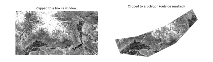
Clipping keeps only your area. With a box, the fastest way is to read just the window of rows and columns that covers it (the file is never read in full). With an irregular area (a catchment, a district) you then mask the pixels outside the polygon. The polygon must be in the same CRS as the raster: convert it first.
The polygon here is drawn by hand around the valley floor between Aliabad and Gulmit, as an example of a study area.
AOI = [74.55, 36.28, 74.95, 36.45]
valley = gpd.GeoDataFrame(geometry=[Polygon([(74.60, 36.30), (74.70, 36.29), (74.80, 36.33), (74.88, 36.40),
                                             (74.86, 36.43), (74.76, 36.38), (74.66, 36.35), (74.58, 36.34)])], crs="EPSG:4326")
with rasterio.open(item.assets["B04"].href) as src:
    win = from_bounds(*transform_bounds("EPSG:4326", src.crs, *AOI), src.transform)
    red = src.read(1, window=win)
    wtf = src.window_transform(win)
    poly = valley.to_crs(src.crs)
    clipped, ctf = rio_mask(src, poly.geometry, crop=True, nodata=0)
print("box window:", red.shape, "| polygon clip:", clipped.shape[1:], "| pixels inside polygon:", int((clipped[0] > 0).sum()))
fig, ax = plt.subplots(1, 2, figsize=(10, 3.6))
ax[0].imshow(red, cmap="gray", vmin=1000, vmax=4000)
ax[0].set_title("Clipped to a box (a window)", fontsize=9)
ax[1].imshow(np.ma.masked_equal(clipped[0], 0), cmap="gray", vmin=1000, vmax=4000)
ax[1].set_title("Clipped to a polygon (outside masked)", fontsize=9)
for a in ax:
    a.set_axis_off()
plt.show()
box window: (1895, 3593) | polygon clip: (1551, 2694) | pixels inside polygon: 1672083
4.4 Reprojection and resampling
To combine data on different grids (a 10 m UTM image and a 30 m DEM in degrees, say) one must be reprojected onto the other's grid. Each new pixel takes its value from the old pixels near its centre, by a resampling rule:
-
nearest neighbour: the closest old pixel. Keeps original values exactly; the only correct choice for categories (land cover classes, masks, quality flags), which must never be averaged.
-
bilinear: a distance-weighted mean of the 4 nearest pixels. Smooth; good for continuous values (reflectance, elevation, temperature).
-
cubic: uses 16 pixels; sharper, but can overshoot past the original range.
-
average: the mean of all old pixels inside each new one; the right choice when making pixels much larger.
Below, the red band is reprojected to geographic coordinates (EPSG:4326) at about 30 m, with each rule, and we compare the statistics. Averaging changes extremes most: bright and dark single pixels are smoothed away.
dst_crs = "EPSG:4326"
tf, w, h = calculate_default_transform(src.crs, dst_crs, red.shape[1], red.shape[0], *rasterio.transform.array_bounds(*red.shape, wtf), resolution=0.0003)
rows = []
for rule in [Resampling.nearest, Resampling.bilinear, Resampling.cubic, Resampling.average]:
    out = np.zeros((h, w), "float32")
    reproject(red.astype("float32"), out, src_transform=wtf, src_crs=src.crs, dst_transform=tf, dst_crs=dst_crs,
              resampling=rule, src_nodata=0, dst_nodata=0)
    v = out[out > 0]
    rows.append(dict(rule=rule.name, pixels=v.size, mean=v.mean(), min=v.min(), max=v.max(), std=v.std()))
v = red[red > 0]
rows.insert(0, dict(rule="original 10 m", pixels=v.size, mean=v.mean(), min=v.min(), max=v.max(), std=v.std()))
pd.DataFrame(rows).round(1)
rule   pixels    mean          min           max     std
0  original 10 m  6808735  3214.9   437.000000  16753.000000  2089.7
1        nearest   760593  3214.9  1012.000000  16751.000000  2090.2
2       bilinear   760593  3215.4  1039.599976  16621.699219  1999.1
3          cubic   760593  3215.4   974.000000  17851.199219  2036.2
4        average   761906  3216.2  1038.400024  16703.900391  2024.4
4.5 Mosaicking: joining tiles
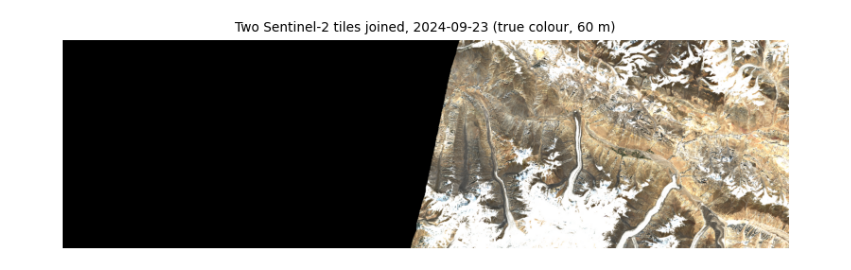
Sentinel-2 is cut into 110 by 110 km tiles on the MGRS grid; Landsat into path/row scenes. An area across a tile boundary needs a mosaic. Tiles from the same orbit and date line up exactly (same sun, same atmosphere); tiles from different dates show seams. Where tiles overlap, a rule decides which value wins: the first tile, the last, or the mean. Here we join two tiles from the same orbit and day.
WIDE = [74.3, 36.3, 75.6, 36.6]                          # wider than one tile: reaches the next tile east
wide_items = catalog.search(collections=["sentinel-2-l2a"], bbox=WIDE, datetime="2024-06-01/2024-09-30",
                            query={"eo:cloud_cover": {"lt": 20}}).items()
by_tile = {}
for i in wide_items:
    by_tile.setdefault(i.properties["datetime"][:10], {})[i.properties["s2:mgrs_tile"]] = i
day, tiles = next((d, t) for d, t in sorted(by_tile.items(), key=lambda kv: -len(kv[1])) if len(t) >= 2)
print("date with", len(tiles), "tiles:", day, sorted(tiles))
srcs = [rasterio.open(t.assets["visual"].href) for t in list(tiles.values())[:2]]
bounds = transform_bounds("EPSG:4326", srcs[0].crs, *WIDE)
mosaic, mtf = merge(srcs, bounds=bounds, res=60, resampling=Resampling.average, method="first", nodata=0)
for s in srcs:
    s.close()
print("mosaic:", mosaic.shape, "(bands, rows, columns) at 60 m")
plt.figure(figsize=(9, 3.2))
plt.imshow(np.moveaxis(mosaic, 0, -1))
plt.title(f"Two Sentinel-2 tiles joined, {day} (true colour, 60 m)", fontsize=9)
plt.axis("off")
plt.show()
date with 2 tiles: 2024-09-23 ['43SDA', '43SEA']
mosaic: (3, 558, 1945) (bands, rows, columns) at 60 m
4.6 Stacking bands of different pixel sizes
Analysis is easiest with all bands in one 3-D array (band, row, column) on one grid. Sentinel-2's bands come at 10, 20 and 60 m, so the 20 m bands are resampled to 10 m (bilinear, since reflectance is continuous) and the 20 m scene classification layer (SCL), which holds categories, with nearest neighbour.
STUDY = [74.60, 36.30, 74.80, 36.42]
def read_to(item, key, bbox, shape, rule):
    with rasterio.open(item.assets[key].href) as s:
        win = from_bounds(*transform_bounds("EPSG:4326", s.crs, *bbox), s.transform)
        return s.read(1, window=win, out_shape=shape, resampling=rule)

with rasterio.open(item.assets["B02"].href) as s:
    win = from_bounds(*transform_bounds("EPSG:4326", s.crs, *STUDY), s.transform)
    shape = s.read(1, window=win).shape
keys = ["B02", "B03", "B04", "B08", "B11", "B12"]
stack = np.stack([read_to(item, k, STUDY, shape, Resampling.bilinear) for k in keys])
scl = read_to(item, "SCL", STUDY, shape, Resampling.nearest)
print("stack:", stack.shape, stack.dtype, "| SCL:", scl.shape, "| SCL classes present:", sorted(np.unique(scl).tolist()))
stack: (6, 1337, 1798) uint16 | SCL: (1337, 1798) | SCL classes present: [2, 3, 4, 5, 6, 7, 8, 9, 11]
4.7 Masking no-data and cloud
Two kinds of pixel must be removed before statistics. No-data pixels (outside the image, value 0 here) carry no measurement. Cloud and cloud shadow hide the ground. Sentinel-2 Level-2A includes the scene classification layer, a per-pixel label from the Sen2Cor processor:
| SCL | Meaning | SCL | Meaning |
|---|---|---|---|
| no data | 6 | water | |
| 1 | saturated or defective | 7 | unclassified |
| 2 | dark area | 8 | cloud, medium probability |
| 3 | cloud shadow | 9 | cloud, high probability |
| 4 | vegetation | 10 | thin cirrus |
| 5 | not vegetated | 11 | snow or ice |
A mask is a true/false array; numpy's where replaces masked values with NaN ("not a number"), which statistics functions such as nanmean skip. Masks are never perfect: SCL confuses bright snow with cloud and dark shadows with water, especially in mountains, so always look at what you remove. In the output below about a sixth of the valley is "dark area": mostly slopes in the shadow of mountains, which the mask keeps, since they are real ground; their values are low because little sunlight reaches them, the topographic effect again.
names = {0: "no data", 1: "saturated", 2: "dark area", 3: "cloud shadow", 4: "vegetation", 5: "not vegetated", 6: "water",
         7: "unclassified", 8: "cloud medium", 9: "cloud high", 10: "cirrus", 11: "snow or ice"}
v, n = np.unique(scl, return_counts=True)
print(pd.Series(n / n.sum() * 100, index=[names[int(x)] for x in v]).round(1).to_string(), "\n(% of pixels)")
bad = np.isin(scl, [0, 1, 3, 8, 9, 10])
refl = np.where(bad[None], np.nan, (stack.astype("float32") - 1000) / 10000)
print("kept", f"{100 * (~bad).mean():.1f}% of pixels")
dark area        16.5
cloud shadow      0.0
vegetation        7.7
not vegetated    52.4
water             0.3
unclassified      0.3
cloud medium      0.1
cloud high        0.0
snow or ice      22.6
(% of pixels)
kept 99.9% of pixels
4.8 Composites over time
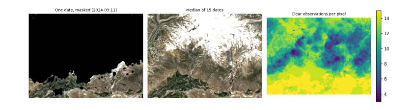
One image is one moment, often with cloud. A composite combines many dates into one cloud-free picture by taking, at each pixel, a statistic over the clear observations. The median is the usual choice: it ignores the few cloudy or shadowed values that slip past the mask, which a mean would not. The cost is that a composite no longer shows one moment, so it suits slowly changing things (land cover) better than quick ones (snow on a given day).
Below, every summer 2024 image of the study area is masked and the median taken. We use the 20 m bands to keep memory low.
use = [i for i in items if i.properties["s2:mgrs_tile"] == item.properties["s2:mgrs_tile"]]
with rasterio.open(item.assets["B11"].href) as s:
    win = from_bounds(*transform_bounds("EPSG:4326", s.crs, *STUDY), s.transform)
    shape20 = s.read(1, window=win).shape
layers, clear = [], []
for it in use:
    s_cl = read_to(it, "SCL", STUDY, shape20, Resampling.nearest)
    ok = ~np.isin(s_cl, [0, 1, 3, 8, 9, 10])
    off = -1000 if float(it.properties["s2:processing_baseline"]) >= 4 else 0
    rgb = np.stack([read_to(it, k, STUDY, shape20, Resampling.average) for k in ["B04", "B03", "B02"]]).astype("float32")
    layers.append(np.where(ok[None], (rgb + off) / 10000, np.nan))
    clear.append(round(float(ok.mean()), 2))
cube = np.stack(layers)                                   # date, band, row, column
median = np.nanmedian(cube, axis=0)
count = np.isfinite(cube[:, 0]).sum(0)
print(len(use), "dates; clear share per date:", clear)
print("clear observations per pixel: min", int(count.min()), "median", int(np.median(count)), "max", int(count.max()))
fig, ax = plt.subplots(1, 3, figsize=(12, 3.6))
show = lambda a: np.clip(np.moveaxis(a, 0, -1) / 0.35, 0, 1)
worst = int(np.argmin(clear))
ax[0].imshow(show(np.nan_to_num(cube[worst], nan=0)))
ax[0].set_title(f"One date, masked ({use[worst].properties['datetime'][:10]})", fontsize=9)
ax[1].imshow(show(np.nan_to_num(median, nan=0)))
ax[1].set_title(f"Median of {len(use)} dates", fontsize=9)
im = ax[2].imshow(count, cmap="viridis")
ax[2].set_title("Clear observations per pixel", fontsize=9)
plt.colorbar(im, ax=ax[2], fraction=0.04)
for a in ax:
    a.set_axis_off()
plt.tight_layout()
plt.show()
15 dates; clear share per date: [0.78, 0.6, 0.64, 0.95, 0.88, 0.95, 1.0, 0.71, 0.82, 0.83, 0.46, 0.88, 0.27, 1.0, 0.72]
clear observations per pixel: min 3 median 12 max 15
4.9 Saving the result properly
A result is only useful if others can open it in any GIS and know what it is. Save rasters as Cloud-Optimised GeoTIFF with the CRS and transform, a no-data value, compression, band descriptions, and a few words of metadata on how it was made. (Reading it back reports the driver as GTiff: a COG is an ordinary GeoTIFF with its internal tiles and overviews arranged for reading over the web.)
with rasterio.open(item.assets["B11"].href) as s:
    crs20, tf20 = s.crs, rasterio.windows.transform(win, s.transform)
profile = dict(driver="COG", dtype="float32", count=3, width=shape20[1], height=shape20[0], crs=crs20,
               transform=tf20, nodata=np.nan, compress="deflate")
with rasterio.open("hunza_median_summer2024.tif", "w", **profile) as dst:
    dst.write(median.astype("float32"))
    for k, name in enumerate(["red", "green", "blue"], 1):
        dst.set_band_description(k, f"{name} surface reflectance")
    dst.update_tags(source="Sentinel-2 L2A via Microsoft Planetary Computer", method=f"per-pixel median of {len(use)} dates, SCL cloud mask",
                    period="2024-06-01/2024-09-30")
with rasterio.open("hunza_median_summer2024.tif") as chk:
    print(chk.profile["driver"], chk.crs, chk.res, chk.count, "bands |", chk.descriptions, "|", chk.tags()["method"])
GTiff EPSG:32643 (20.0, 20.0) 3 bands | ('red surface reflectance', 'green surface reflectance', 'blue surface reflectance') | per-pixel median of 15 dates, SCL cloud mask
4.10 What to remember
-
Know your CRS, and convert vectors to the raster's CRS, not the other way round, unless you mean to resample.
-
Read only the window you need; clip to polygons after.
-
Nearest neighbour for categories, bilinear or average for continuous values.
-
Mask no-data and cloud before any statistic, and look at what the mask removed.
-
A median composite gives a clear picture of a season, at the cost of losing the moment.
-
Save with CRS, no-data, descriptions and a record of how the file was made.
Exercises. (1) Repeat the composite with the mean instead of the median and find where they differ most. (2) Reproject the composite to UTM zone 43 at 30 m with each resampling rule and compare. (3) Draw a polygon around your own study area and compute the share of clear observations inside it per month.