The whole guide on one page
1. Before you start
This guide is a course in the basics of remote sensing and GIS, built from five notebooks you run yourself. It starts where every real project starts, with getting the data: making accounts, keeping keys safe and downloading in bulk from NASA, Copernicus, Google Earth Engine and open catalogues. It then works through what a satellite measures, how images are prepared, what terrain does to them, and how pixels become maps, numbers and trends. Every example uses real data over one place, the Hunza valley in the Karakoram, where snow, glaciers, bare rock, fields, villages and a large river lie within a few kilometres of each other, and where the ground rises more than 5,000 metres.
It continues the Py4Geo tutorials and the guide Satellite images in Python, which cover rasters, vectors, indices and clustering on a Sentinel-2 image of Belfast. This guide goes further back (accounts, physics, preparation) and further on (terrain, accuracy, time series), and can be read on its own.
1.1 Who it is for
Undergraduates in geography, environmental and Earth sciences, ecology and engineering meeting remote sensing for the first time, and anyone revising the basics. Where an idea from school or first-year science is needed (the speed of light, Planck’s law, a lapse rate, why chlorophyll absorbs red, how a trend test works) it is explained where it is used, with the formula and a numerical check. No programming beyond a first course in Python is assumed: each code cell says what it does and why.
1.2 What you will learn
-
Getting data: who holds which data; accounts and licences; keeping passwords and keys out of code; plain web downloads, STAC catalogues, NASA Earthdata, the Copernicus data stores and Google Earth Engine; bulk downloads that resume, retry and keep a record.
-
Physics: light as wave and photon; Planck’s, Wien’s and the Stefan-Boltzmann laws; atmospheric windows and scattering; bands and the four resolutions; digital numbers, scale factors and reflectance; histograms, stretches, composites and spectral signatures; what atmospheric correction changes.
-
Preparation: projections and transforms; clipping; reprojection and the choice of resampling; mosaics; stacks; no-data and cloud masks; median composites; saving files others can use.
-
Terrain: how DEMs are made and what their heights mean; slope and aspect by finite differences; hillshade; illumination and topographic correction; elevation bands, hypsometry, profiles and lapse rates; a little geomorphology and tectonics.
-
Analysis: indices and the chemistry behind them; thresholds, clustering and a random forest; confusion matrices and honest testing; sieving, vectorising and areas; a time series with the Mann-Kendall test; making a readable map.
1.3 Running the notebooks
Each chapter is one notebook. Open the Notebooks page and choose Open in Colab, or download the .ipynb file. The first cell of each installs what Colab lacks. On your own computer:
conda create -n rs python=3.12 numpy pandas matplotlib scipy scikit-learn xarray netcdf4 rasterio geopandas pystac-client planetary-computer earthaccess cdsapi earthengine-api pyhdf jupyterlab
conda activate rs
jupyter lab
Chapters 2 to 5 need no account: their images come from Microsoft’s Planetary Computer. Chapter 1 shows how to set up NASA Earthdata, Copernicus and Earth Engine, and its cells skip politely where an account is missing; so do the few later cells that use Earth Engine. Boxes labelled In [n] are code and Out [n] what it printed or drew; the outputs shown were made by running the notebooks, with real accounts, in November 2026. Images are read over the internet, so allow a few minutes per notebook.
1.4 Good practice throughout
-
Look before you compute: read metadata, plot histograms, check coded values.
-
Check against known answers: every formula here is tested on a case whose answer is known (a plane of known slope, Wien’s law against the Planck curve, a hand-computed test statistic against a library).
-
Say what you did: versions, dates, thresholds, licences, citations, in a manifest or a methods section.
-
Report uncertainty: accuracies with their confusion matrix, trends with their test and their limits.
2. Getting the data
2.1 Overview
Most of remote sensing starts long before any image is analysed: you need to know who holds the data, how to get permission, and how to download a lot of it reliably. This notebook walks through the services used most in Earth observation and climate science, with working code for each, and the habits that make downloads repeatable.
What you will learn:
-
the difference between open data that needs no account, data behind a free login, and data you process in the cloud instead of downloading;
-
where to keep passwords and keys so that they never end up in a notebook, a repository or a screenshot;
-
five ways of getting data, each with a real example: a plain web download, a STAC catalogue search, NASA Earthdata, the Copernicus data stores (ERA5, GloFAS) and Google Earth Engine;
-
how to download in bulk without losing work: one file per request, skipping what is already there, waiting and retrying when a server says too many requests, checking file sizes and checksums, and keeping a record of every file and its licence.
Everything here runs in Google Colab or on your own computer. Cells that need an account check first and explain what to do if you have not set one up yet, so the notebook runs to the end either way. The outputs shown were made with real accounts.
Libraries. requests downloads over the web; pystac-client and planetary-computer search image catalogues; earthaccess handles NASA Earthdata; cdsapi the Copernicus data stores; earthengine-api Google Earth Engine; xarray and netCDF4 read gridded climate files; pandas keeps tables; matplotlib draws.
import importlib.util, subprocess, sys
need = {"pystac_client": "pystac-client", "planetary_computer": "planetary-computer", "earthaccess": "earthaccess",
        "cdsapi": "cdsapi", "ee": "earthengine-api", "rasterio": "rasterio", "netCDF4": "netCDF4"}
missing = [pkg for mod, pkg in need.items() if importlib.util.find_spec(mod) is None]
if missing:
    subprocess.run([sys.executable, "-m", "pip", "install", "-q", *missing], check=True)

import hashlib, json, os, time
from pathlib import Path
import numpy as np
import pandas as pd
import requests
import xarray as xr
import matplotlib.pyplot as plt
plt.rcParams.update({"figure.dpi": 110})
DATA = Path("rs_data")            # everything this notebook downloads goes here
DATA.mkdir(exist_ok=True)
print("Python", sys.version.split()[0], "| data folder:", DATA.resolve().name)
Python 3.12.12 | data folder: rs_data
2.2 Who holds the data
Satellite and climate data are produced by space agencies and weather centres and handed out through data portals. Most are free; many ask you to register so they can count users, apply a licence, and limit how much one person downloads at once. The table lists the services this guide uses.
Service |
Who runs it |
What you get there |
Account |
How to reach it from code |
|---|---|---|---|---|
NOAA NCEI |
US National Oceanic and Atmospheric Administration |
climate data records, e.g. snow cover since 1966 |
none |
plain web download |
Microsoft Planetary Computer, Earth Search (AWS) |
Microsoft; Element 84 on Amazon |
Sentinel-2, Landsat, Copernicus DEM as cloud-optimised files |
none for reading |
STAC search (pystac-client) |
NASA Earthdata |
NASA |
MODIS, VIIRS, Landsat, GEDI, ICESat-2, SMAP and more |
free login |
earthaccess |
Copernicus Data Space Ecosystem |
European Space Agency and Commission |
all Sentinel missions |
free login |
STAC, OData, S3 |
Copernicus Climate Data Store (CDS) |
ECMWF for the EU |
ERA5 and ERA5-Land reanalysis, satellite climate records |
free login + licence per dataset |
cdsapi |
Copernicus Early Warning Data Store (EWDS) |
ECMWF for the EU |
GloFAS river discharge, EFAS, fire danger |
same login as CDS + its own terms |
cdsapi pointed at the EWDS |
Google Earth Engine |
a catalogue of petabytes processed on Google's computers |
free for research and teaching, with a Cloud project |
earthengine-api |
|
USGS EarthExplorer |
US Geological Survey |
Landsat archive, aerial photos, older DEMs |
free login |
web, or the M2M interface |
Licences. Open does not mean without conditions. Copernicus data must be credited ("Contains modified Copernicus Climate Change Service information [year]"), NASA asks for the dataset's DOI to be cited, and Earth Engine's free tier is for non-commercial use. Note the licence of every dataset when you download it (the last section shows how).
Why so many services? Each agency publishes its own missions. Catalogue standards such as STAC and tools such as earthaccess are slowly making them look alike, which is why the same few lines of code now work for many of them.
2.3 Keeping passwords and keys safe
A password proves who you are when you log in by hand. Programs instead use a token or API key: a long random string the service gives you, which you can cancel at any time without changing your password. Both are secrets. The rules below are the same in every company and research group.
-
Never type a secret into a notebook or script. Notebooks are shared, uploaded and screenshotted; a key in a cell will leak.
-
Keep secrets in a file in your home folder, which is where the tools look for them anyway:
Service |
File |
What it contains |
|---|---|---|
NASA Earthdata |
|
|
Copernicus CDS and EWDS |
|
|
Google Earth Engine |
a credentials file written by |
a refresh token, never typed by you |
-
Or use environment variables, which a program reads but which never appear in the code. In Colab, use the Secrets panel (the key icon) and read them with
google.colab.userdata.get("NAME"). -
Tell git to ignore credential and data files. Add lines such as
.netrc,*.cdsapirc,.envandrs_data/to.gitignore. If a key is ever committed, cancel it on the service's website at once: deleting the commit is not enough, because copies already exist. -
Print what you got, not how you got it. A good log says "downloaded 365 files, 1.1 GB"; it never prints the key, the full home-folder path or the user name.
The cell below checks which of the three credential files exist on this computer, without reading or printing them.
HOME = Path.home()
creds = {
    "NASA Earthdata (.netrc)": (HOME / ".netrc").exists() or (HOME / "_netrc").exists(),
    "Copernicus CDS/EWDS (.cdsapirc)": (HOME / ".cdsapirc").exists(),
    "Earth Engine (credentials)": (HOME / ".config" / "earthengine" / "credentials").exists(),
}
for name, ok in creds.items():
    print(f"{name:34s} {'found' if ok else 'not set up: the cells that need it will explain and skip'}")
HAVE_EARTHDATA, HAVE_CDS, HAVE_EE = creds.values()
NASA Earthdata (.netrc)            found
Copernicus CDS/EWDS (.cdsapirc)    found
Earth Engine (credentials)         found
2.4 Signing up, step by step
You do this once, by hand, in a web browser. Use your university e-mail: some services give academic users more capacity, and it makes clear the use is non-commercial.
NASA Earthdata. Go to urs.earthdata.nasa.gov, choose Register, fill in the form and confirm your e-mail. Then store the login for programs. The simplest way is to let earthaccess write the .netrc file for you, in a terminal (not in a shared notebook): python -c "import earthaccess; earthaccess.login(strategy='interactive', persist=True)". It asks for the user name and password and saves them in your home folder.
Copernicus Climate Data Store. Register at cds.climate.copernicus.eu (one ECMWF account works for the CDS, the Atmosphere Data Store and the Early Warning Data Store). Your API token is on your profile page. Create the file .cdsapirc in your home folder with two lines, url: https://cds.climate.copernicus.eu/api and key: followed by the token. Each dataset has a licence that you accept once on its Download tab; a request for a dataset whose licence you have not accepted fails with a message naming it. The EWDS also has its own terms of use to accept.
Google Earth Engine. Go to earthengine.google.com, choose Get started, and register a Google Cloud project for non-commercial use (research or teaching). The project's ID (for example ee-yourname) is passed to every session. Then run earthengine authenticate once in a terminal, or ee.Authenticate() in Colab; a browser window asks you to allow access and stores a token.
Copernicus Data Space Ecosystem (for Sentinel files) is at dataspace.copernicus.eu; registration works the same way. This notebook reads Sentinel-2 through the Planetary Computer instead, which needs no account.
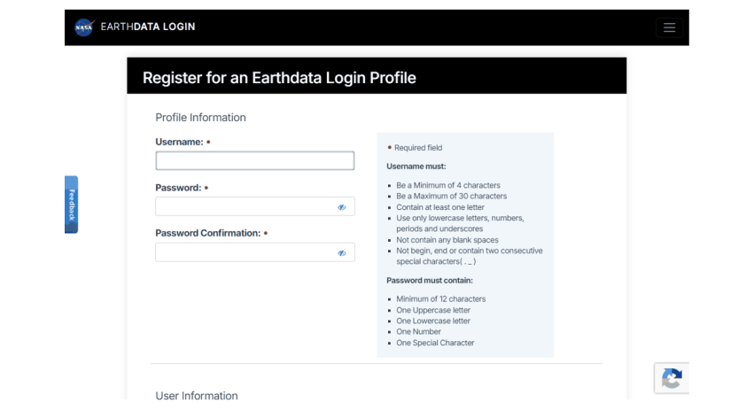
The NASA Earthdata registration form (urs.earthdata.nasa.gov).
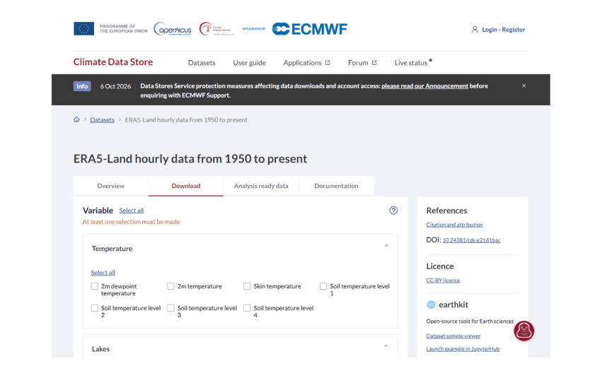
A Climate Data Store dataset page: the Download tab builds a request; the right column gives the DOI to cite and the licence to accept.
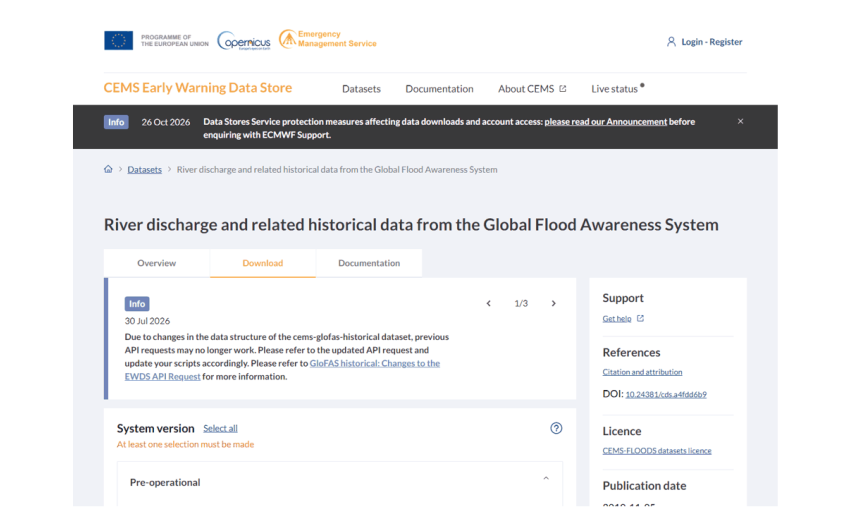
GloFAS on the Early Warning Data Store, with the notice that its request format changed in 2026.
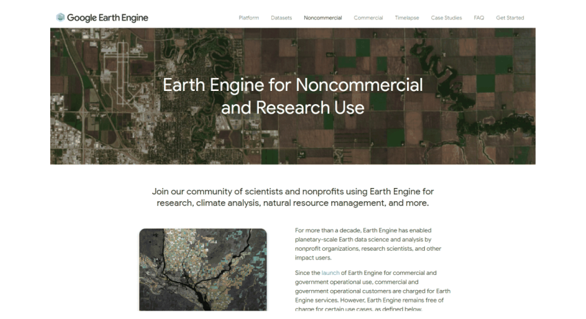
Google Earth Engine’s page for non-commercial and research use.
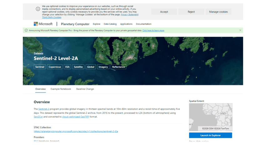
A dataset page on Microsoft’s Planetary Computer, which gives the STAC address used in code.
2.5 Method 1: a plain web download
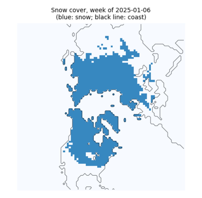
Some data need nothing but a web address. NOAA's Climate Data Record of Northern Hemisphere snow cover is one file, updated weekly, with every week's snow map since October 1966. Three habits make even a single download robust:
-
stream the file to disk in pieces instead of holding it all in memory;
-
check the size against what the server announced (the
Content-Lengthheader), so a broken connection is not mistaken for a finished file; -
write to a temporary name and rename only when complete, so a half-written file never looks finished.
A checksum (here SHA-256) is a short fingerprint of a file's contents; if one byte changes, the fingerprint changes. Recording it lets anyone confirm later that they have exactly the file you used.
def download(url, dest, chunk=1 << 20, session=None):
    """Download url to dest unless it is already there and complete. Returns (path, size in bytes, sha256)."""
    s = session or requests.Session()
    dest = Path(dest)
    head = s.head(url, allow_redirects=True, timeout=60)
    size = int(head.headers.get("Content-Length", 0))
    if not (dest.exists() and size and dest.stat().st_size == size):
        tmp = dest.with_suffix(dest.suffix + ".part")
        with s.get(url, stream=True, timeout=120) as r:
            r.raise_for_status()
            with open(tmp, "wb") as f:
                for block in r.iter_content(chunk):
                    f.write(block)
        if size and tmp.stat().st_size != size:
            raise IOError(f"incomplete: {tmp.stat().st_size} of {size} bytes")
        tmp.replace(dest)
    h = hashlib.sha256()
    with open(dest, "rb") as f:
        for block in iter(lambda: f.read(chunk), b""):
            h.update(block)
    return dest, dest.stat().st_size, h.hexdigest()

index = requests.get("https://www.ncei.noaa.gov/data/snow-cover-extent/access/", timeout=60).text
name = sorted(set(pd.Series(index.split('"')).loc[lambda s: s.str.startswith("nhsce_") & s.str.endswith(".nc")]))[-1]
path, nbytes, sha = download(f"https://www.ncei.noaa.gov/data/snow-cover-extent/access/{name}", DATA / name)
print(f"{path.name}: {nbytes / 1e6:.1f} MB, sha256 {sha[:16]}...")
nhsce_v01r01_19661004_20261102.nc: 24.7 MB, sha256 c758f2764172f8b9...
Now look inside. The file is NetCDF, the usual format for gridded climate data: named variables on named axes (here time, y and x), with attributes that describe units, meanings and the licence. Reading the attributes before the numbers is a habit worth forming: this one tells us snow is coded 1, no snow 0, and that -127 marks missing weeks.
ds = xr.open_dataset(path, mask_and_scale=False)
v = ds.snow_cover_extent
print(ds.sizes)
print("meaning of values:", dict(zip(v.attrs["flag_values"].tolist(), v.attrs["flag_meanings"].split())))
vals, counts = np.unique(v.values, return_counts=True)
print("values actually present:", dict(zip(vals.tolist(), counts.tolist())), "  <- -127 is not in the list above")
print("licence:", ds.attrs.get("license"), "| cite:", ds.attrs.get("metadata_link"))
Frozen({'x': 88, 'y': 88, 'time': 3135})
meaning of values: {0: 'no_snow', 1: 'snow_covered'}
values actually present: {-127: 286528, 0: 21762862, 1: 2228050}   <- -127 is not in the list above
licence: No restrictions on access or use | cite: https://doi.org/10.7289/V5N014G9
week = v.sel(time="2025-01-06", method="nearest")
fig, ax = plt.subplots(figsize=(4.5, 4.5))
ax.imshow(np.where(week.values < 0, np.nan, week.values), cmap="Blues", vmin=0, vmax=1.5)
ax.contour(ds.land.values, levels=[0.5], colors="black", linewidths=0.4)
ax.set_title(f"Snow cover, week of {str(week.time.values)[:10]}\n(blue: snow; black line: coast)", fontsize=9)
ax.set_axis_off()
plt.show()
2.6 Method 2: searching a STAC catalogue
Large image archives are now described by STAC, the SpatioTemporal Asset Catalog standard. A catalogue holds collections (for example Sentinel-2 Level-2A); each collection holds items (one image of one place at one time); each item lists assets (one file per band, plus thumbnails and metadata). Because the format is shared, the same search works on the Planetary Computer, Earth Search, the Copernicus Data Space and many others.
The files are Cloud-Optimised GeoTIFFs (COGs): ordinary GeoTIFFs arranged so a program can fetch only the part it needs over the web. Below we search for Sentinel-2 images of the Hunza valley in the Karakoram and read a small window of one band without downloading the 100 km tile.
import pystac_client, planetary_computer, rasterio
from rasterio.windows import from_bounds
from rasterio.warp import transform_bounds

catalog = pystac_client.Client.open("https://planetarycomputer.microsoft.com/api/stac/v1",
                                    modifier=planetary_computer.sign_inplace)
BBOX = [74.55, 36.25, 74.75, 36.40]              # west, south, east, north: Karimabad and the Hunza valley
search = catalog.search(collections=["sentinel-2-l2a"], bbox=BBOX, datetime="2025-03-01/2025-04-30",
                        query={"eo:cloud_cover": {"lt": 15}})
items = sorted(search.items(), key=lambda i: i.properties["eo:cloud_cover"])
print(len(items), "images; clearest:", items[0].id, "| cloud", round(items[0].properties["eo:cloud_cover"], 1), "%")
print("assets:", ", ".join(list(items[0].assets)[:16]), "...")
3 images; clearest: S2B_MSIL2A_20250429T054639_R048_T43SDA_20250429T075112 | cloud 0.0 %
assets: AOT, B01, B02, B03, B04, B05, B06, B07, B08, B09, B11, B12, B8A, SCL, WVP, visual ...
item = items[0]
with rasterio.open(item.assets["B03"].href) as src:
    win = from_bounds(*transform_bounds("EPSG:4326", src.crs, *BBOX), src.transform)
    green = src.read(1, window=win)
    print("file CRS:", src.crs, "| pixel size:", src.res, "m | window:", green.shape, "pixels",
          f"(read {green.nbytes / 1e6:.1f} MB of a {src.width} x {src.height} tile)")
file CRS: EPSG:32643 | pixel size: (10.0, 10.0) m | window: (1670, 1801) pixels (read 6.0 MB of a 10980 x 10980 tile)
2.7 Method 3: NASA Earthdata with earthaccess
NASA's archives (at the NSIDC, LP DAAC, GES DISC and others) share one login, Earthdata Login, and one search system, CMR (the Common Metadata Repository). The earthaccess library wraps both: search needs no login, download does. Here we look for MOD10A1F, MODIS daily snow cover with cloud gaps filled from the last clear view, for the MODIS tile h24v05 (the Karakoram).
MODIS data come in tiles on a sinusoidal grid, named by column (h) and row (v); each tile is about 1,100 km across and holds 2,400 by 2,400 pixels of 500 m. Files are HDF4, an older scientific format holding several named datasets.
import earthaccess
granules = earthaccess.search_data(short_name="MOD10A1F", version="61", granule_name="*h24v05*",
                                   temporal=("2024-01-01", "2024-01-31"))
sizes = [g.size() for g in granules]
print(len(granules), "daily files for January 2024;", f"{sum(sizes):.0f} MB in total;",
      f"a full year would be about {np.mean(sizes) * 365 / 1000:.1f} GB")
print("first file:", granules[0].data_links()[0].split("/")[-1])
31 daily files for January 2024; 80 MB in total; a full year would be about 0.9 GB
first file: MOD10A1F.A2024001.h24v05.061.2024005105118.hdf
if HAVE_EARTHDATA:
    earthaccess.login(strategy="netrc")
    files = earthaccess.download(granules[:1], str(DATA / "mod10a1f"))
    from pyhdf.SD import SD, SDC
    hdf = SD(str(files[0]), SDC.READ)
    print("datasets in the file:", list(hdf.datasets()))
    snow = hdf.select("CGF_NDSI_Snow_Cover")[:]
    print("array:", snow.shape, snow.dtype)
else:
    print("No Earthdata login on this computer: see 'Signing up, step by step'. Search worked; download skipped.")
QUEUEING TASKS | :   0%|          | 0/1 [00:00<?, ?it/s]
PROCESSING TASKS | :   0%|          | 0/1 [00:00<?, ?it/s]
COLLECTING RESULTS | :   0%|          | 0/1 [00:00<?, ?it/s]
datasets in the file: ['CGF_NDSI_Snow_Cover', 'Cloud_Persistence', 'Basic_QA', 'Algorithm_Flags_QA', 'MOD10A1_NDSI_Snow_Cover']
array: (2400, 2400) uint8
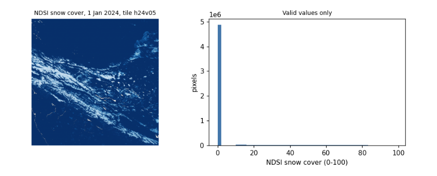
Reading the values. The product stores the NDSI snow cover, 0 to 100, and codes above 100 for things that are not snow measurements: 237 inland water, 239 ocean, 250 cloud (rare here, since gaps were filled), 255 fill. Treating those codes as numbers is one of the commonest mistakes in remote sensing: always mask them before averaging. The histogram shows the range of valid values.
if HAVE_EARTHDATA:
    valid = snow[snow <= 100]
    codes, n = np.unique(snow[snow > 100], return_counts=True)
    print("coded (non-measurement) values:", dict(zip(codes.tolist(), n.tolist())))
    fig, ax = plt.subplots(1, 2, figsize=(9, 3.6))
    ax[0].imshow(np.ma.masked_greater(snow, 100), cmap="Blues_r")
    ax[0].set_title("NDSI snow cover, 1 Jan 2024, tile h24v05", fontsize=9)
    ax[0].set_axis_off()
    ax[1].hist(valid, bins=50, color="#4477aa")
    ax[1].set_xlabel("NDSI snow cover (0-100)")
    ax[1].set_ylabel("pixels")
    ax[1].set_title("Valid values only", fontsize=9)
    plt.tight_layout()
    plt.show()
coded (non-measurement) values: {237: 17689}
2.8 Method 4: the Copernicus data stores with cdsapi
ECMWF runs several data stores with the same interface: the Climate Data Store (ERA5, ERA5-Land), the Atmosphere Data Store (air quality) and the Early Warning Data Store (GloFAS river discharge, EFAS). You do not download a file that already exists: you send a request naming the dataset, variables, dates and area, the store builds the file, and you download it when it is ready. Requests wait in a queue, so large ones can take hours.
Finding the right options. Every dataset publishes the combinations it accepts (its constraints). Option names change between versions: in 2025 GloFAS renamed hyear to year and its discharge variable to average_river_discharge_in_the_last_24_hours, and moved from the CDS to the EWDS. When a request fails with not a valid combination, read the constraints rather than guessing, as the next cell does.
meta = requests.get("https://ewds.climate.copernicus.eu/api/catalogue/v1/collections/cems-glofas-historical", timeout=60).json()
link = next(l["href"] for l in meta["links"] if l["rel"] == "constraints")
cons = requests.get(link, timeout=60).json()
opts = {}
for c in cons:
    for k, vals in c.items():
        opts.setdefault(k, set()).update(vals)
for k in ["system_version", "product_type", "variable", "timespan", "hydrological_model"]:
    print(f"{k:20s}", sorted(opts[k]))
print("years available:", min(opts["year"]), "to", max(opts["year"]))
system_version       ['version_4_0', 'version_5_0']
product_type         ['consolidated', 'intermediate']
variable             ['average_river_discharge_in_the_last_24_hours', 'runoff_water_equivalent', 'snow_depth_water_equivalent', 'soil_wetness_index']
timespan             ['instantaneous', 'time_mean']
hydrological_model   ['lisflood']
years available: 1979 to 2026
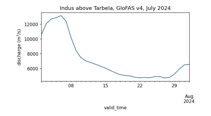
The request below asks for one month of daily river discharge from GloFAS v4 over a small box on the Indus between Besham Qila and Tarbela reservoir; the cell with the largest mean flow is the main channel. (A version 5 also appears in the constraints above; whichever you use, name it in your methods, since versions differ.) GloFAS is a hydrological model (LISFLOOD) driven by ERA5 weather, not a measurement: it gives discharge on a 0.05 degree grid everywhere, which makes it useful where gauge records are not public, but it must be checked against gauges before its absolute values are trusted.
if HAVE_CDS:
    import cdsapi
    key = [l.split(":", 1)[1].strip() for l in (HOME / ".cdsapirc").read_text().splitlines() if l.startswith("key")][0]
    ewds = cdsapi.Client(url="https://ewds.climate.copernicus.eu/api", key=key, quiet=True, progress=False)
    target = DATA / "glofas_indus_2024_07.nc"
    if not target.exists():
        ewds.retrieve("cems-glofas-historical", {
            "system_version": ["version_4_0"], "hydrological_model": ["lisflood"], "product_type": ["consolidated"],
            "variable": ["average_river_discharge_in_the_last_24_hours"], "timespan": ["time_mean"],
            "year": ["2024"], "month": ["07"], "day": [f"{d:02d}" for d in range(1, 32)],
            "data_format": "netcdf", "download_format": "unarchived", "area": [35.2, 72.6, 34.7, 73.1]}, str(target))
    q = xr.open_dataset(target)
    dis = q[[n for n in q.data_vars if q[n].ndim == 3][0]]
    mean = dis.mean(dis.dims[0])
    lat, lon = np.unravel_index(int(mean.argmax()), mean.shape)        # the main channel carries the most water
    series = dis.isel(latitude=lat, longitude=lon).to_series()
    print(f"cell {float(q.latitude[lat]):.3f} N, {float(q.longitude[lon]):.3f} E;",
          f"July 2024 mean {series.mean():,.0f} m3/s, peak {series.max():,.0f} m3/s")
    series.plot(figsize=(6, 2.8), color="#4477aa", ylabel="discharge (m$^3$/s)", title="Indus above Tarbela, GloFAS v4, July 2024")
    plt.show()
else:
    print("No ~/.cdsapirc on this computer: see 'Signing up, step by step'.")
cell 34.725 N, 72.825 E; July 2024 mean 7,152 m3/s, peak 13,167 m3/s
2.9 Method 5: Google Earth Engine
Earth Engine turns the problem around: instead of downloading the data to your computer, you send your program to the data. The code you write builds a description of a calculation; nothing runs until you ask for a result (getInfo()), a picture, or an export (a file written to Google Drive, Cloud Storage or an Earth Engine asset).
Three limits shape how you work with it:
-
an interactive request must finish within about five minutes, or it fails with computation timed out;
-
very long chains of steps fail with computation is too complex (a loop over hundreds of days, for example): split the work, or export it as a batch task, which runs for hours in the background;
-
the free non-commercial tier limits how many requests run at once. Too many fail with Too Many Requests; the cure is to wait and retry, as the last section shows.
EE_PROJECT = os.environ.get("EE_PROJECT")           # your Cloud project ID, e.g. set in a terminal: EE_PROJECT=ee-yourname
if HAVE_EE and EE_PROJECT:
    import ee
    ee.Initialize(project=EE_PROJECT)
    hunza = ee.Geometry.Rectangle(BBOX)
    col = ee.ImageCollection("MODIS/061/MOD10A1").filterDate("2024-10-01", "2025-10-01").select("NDSI_Snow_Cover")
    snow_days = col.map(lambda i: i.gte(40).unmask(0)).sum()            # days with snow
    clear_days = col.map(lambda i: i.mask().gt(0)).sum()                # days with a clear view
    stats = snow_days.rename("snow_days").addBands(clear_days.rename("clear_days")).reduceRegion(ee.Reducer.mean(), hunza, 500)
    print("Hunza valley box, October 2024 to September 2025, mean per pixel:", {k: round(v, 1) for k, v in stats.getInfo().items()})
    print("images in the collection:", col.size().getInfo())
else:
    print("Earth Engine not set up here: register a Cloud project, run 'earthengine authenticate',",
          "and set EE_PROJECT to the project ID.")
Hunza valley box, October 2024 to September 2025, mean per pixel: {'clear_days': 177.8, 'snow_days': 21.3}
images in the collection: 365
2.10 Downloading in bulk
Research needs hundreds or thousands of files. Five habits make that safe:
-
One request per file, small enough to finish in minutes (a month, a year, a tile). A failure then costs one piece, not the whole job.
-
Skip what is already done, so the same script can simply be run again after an interruption.
-
Wait and retry when a server refuses with a temporary error (HTTP 429 too many requests, 503 unavailable), waiting longer each time (exponential backoff). Never retry at once in a tight loop: it makes the problem worse and can get your account blocked.
-
Check every file (size, and that it opens) before counting it as done.
-
Write a manifest: a table of every file with its source, date, size and checksum, and the dataset's licence and citation. It is what makes your data section reproducible.
The function below combines habits 2 to 4 for any download function; the next cell uses it to fetch three months of GloFAS and writes the manifest.
def with_retries(fn, *args, tries=6, wait=10, **kw):
    """Call fn; on a temporary failure wait 10, 20, 40... seconds and try again."""
    for attempt in range(tries):
        try:
            return fn(*args, **kw)
        except Exception as e:                                            # narrow this to the library's own errors in real code
            temporary = any(s in str(e) for s in ("429", "503", "Too Many Requests", "timed out", "Connection"))
            if not temporary or attempt == tries - 1:
                raise
            print(f"  temporary failure ({str(e)[:60]}...), waiting {wait * 2 ** attempt} s")
            time.sleep(wait * 2 ** attempt)

def sha256(p):
    return hashlib.sha256(Path(p).read_bytes()).hexdigest()

manifest = []
if HAVE_CDS:
    for month in ["05", "06", "07"]:
        target = DATA / f"glofas_indus_2024_{month}.nc"
        if not target.exists():                                           # habit 2: skip what is done
            with_retries(ewds.retrieve, "cems-glofas-historical", {
                "system_version": ["version_4_0"], "hydrological_model": ["lisflood"], "product_type": ["consolidated"],
                "variable": ["average_river_discharge_in_the_last_24_hours"], "timespan": ["time_mean"],
                "year": ["2024"], "month": [month], "day": [f"{d:02d}" for d in range(1, 32)],
                "data_format": "netcdf", "download_format": "unarchived", "area": [35.2, 72.6, 34.7, 73.1]}, str(target))
        xr.open_dataset(target).close()                                   # habit 4: it opens
        manifest.append(dict(file=target.name, source="Copernicus EWDS, cems-glofas-historical v4.0",
                             bytes=target.stat().st_size, sha256=sha256(target)[:16],
                             licence="CEMS-FLOODS data licence", cite="doi:10.24381/cds.a4fdd6b9"))
manifest.append(dict(file=path.name, source="NOAA NCEI snow cover extent CDR v01r01", bytes=nbytes, sha256=sha[:16],
                     licence="no restrictions", cite="doi:10.7289/V5N014G9"))
manifest = pd.DataFrame(manifest)
manifest.to_csv(DATA / "manifest.csv", index=False)
manifest
file  \
0            glofas_indus_2024_05.nc
1            glofas_indus_2024_06.nc
2            glofas_indus_2024_07.nc
3  nhsce_v01r01_19661004_20261102.nc

                                         source     bytes            sha256  \
0  Copernicus EWDS, cems-glofas-historical v4.0     30501  363a8fa79dfe6da3
1  Copernicus EWDS, cems-glofas-historical v4.0     30502  723225237fe1e2f0
2  Copernicus EWDS, cems-glofas-historical v4.0     30891  c097fe52f94d2d7b
3        NOAA NCEI snow cover extent CDR v01r01  24671777  c758f2764172f8b9

                    licence                       cite
0  CEMS-FLOODS data licence  doi:10.24381/cds.a4fdd6b9
1  CEMS-FLOODS data licence  doi:10.24381/cds.a4fdd6b9
2  CEMS-FLOODS data licence  doi:10.24381/cds.a4fdd6b9
3           no restrictions       doi:10.7289/V5N014G9
2.11 What to remember
-
Find out who holds a dataset, what licence it carries and how it is reached (plain web, STAC, earthaccess, cdsapi, Earth Engine) before writing any analysis.
-
Keep secrets out of code: credential files in your home folder, environment variables, Colab Secrets.
-
Read the metadata of every file first: units, coded values, missing-data markers, licence.
-
Read only the part you need (COG windows, small request areas), and download in pieces that can be skipped, retried and checked.
-
Keep a manifest. Your methods section, and anyone repeating your work, will need it.
Exercises. (1) Change the STAC search to Landsat (landsat-c2-l2) and compare how many images each mission has for the same months. (2) Use earthaccess to count MOD10A1F files for a whole year and estimate the download size for the tiles covering your own country. (3) Request ERA5-Land monthly 2 m temperature (reanalysis-era5-land-monthly-means) for a box of your choice, and add it to the manifest with its licence and citation.
3. What a satellite measures
3.1 Overview
A satellite image is a grid of measurements of light: how much electromagnetic energy reached the sensor from each patch of ground, in a few narrow ranges of wavelength called bands. To read an image well you need a little physics (what light is and where it comes from), a little chemistry and biology (why snow, leaves, water and rock reflect differently) and a little arithmetic (how the numbers in the file become physical quantities).
This notebook builds that up from first principles and checks each idea on a real image: Sentinel-2 over the Hunza valley in the Karakoram in spring, with snow, glaciers, bare rock, villages, orchards and a river in one scene.
What you will learn: waves and photons; Planck's law and why the Sun and the Earth are seen in different bands; the atmosphere's windows; bands and the four kinds of resolution; digital numbers, scale factors and reflectance; histograms and contrast stretches; true- and false-colour composites; spectral signatures; and what atmospheric correction changes.
import importlib.util, subprocess, sys
need = {"pystac_client": "pystac-client", "planetary_computer": "planetary-computer", "rasterio": "rasterio"}
missing = [p for m, p in need.items() if importlib.util.find_spec(m) is None]
if missing:
    subprocess.run([sys.executable, "-m", "pip", "install", "-q", *missing], check=True)
import numpy as np
import pandas as pd
import matplotlib.pyplot as plt
import pystac_client, planetary_computer, rasterio
from rasterio.windows import from_bounds
from rasterio.warp import transform_bounds
from rasterio.enums import Resampling
plt.rcParams.update({"figure.dpi": 110})
3.2 Light as a wave and as a particle
Light is an electromagnetic wave: electric and magnetic fields oscillating together, travelling at the speed of light \(c \approx 3.00 \times 10^8\) m/s in a vacuum. Its wavelength \(\lambda\) (distance between crests) and frequency \(\nu\) (crests per second) are tied by
Light also arrives in packets, photons, each carrying energy
where \(h = 6.626 \times 10^{-34}\) J s is Planck's constant. Shorter wavelength means more energy per photon: an ultraviolet photon can break chemical bonds (sunburn), an infrared one only warms. Remote sensing uses wavelengths from about 0.4 micrometres (\(\mu\)m, millionths of a metre; visible light) to about 1 metre (radar).
Region |
Wavelength |
Used for |
|---|---|---|
visible (blue, green, red) |
to 0.7 m |
colour images, water, sediment |
near infrared (NIR) |
to 1.3 m |
vegetation |
shortwave infrared (SWIR) |
to 3 m |
snow versus cloud, moisture, minerals |
thermal infrared (TIR) |
to 14 m |
surface temperature |
microwave (radar) |
mm to 1 m |
through cloud, day and night; roughness and moisture |
h, c, k = 6.62607015e-34, 2.99792458e8, 1.380649e-23        # Planck, speed of light, Boltzmann (exact SI values)
for name, lam in [("blue", 0.49e-6), ("near infrared", 0.84e-6), ("shortwave infrared", 1.61e-6), ("thermal", 10.9e-6), ("radar C-band", 0.055)]:
    print(f"{name:20s} wavelength {lam:9.2e} m   frequency {c / lam:9.2e} Hz   photon energy {h * c / lam:9.2e} J")
blue                 wavelength  4.90e-07 m   frequency  6.12e+14 Hz   photon energy  4.05e-19 J
near infrared        wavelength  8.40e-07 m   frequency  3.57e+14 Hz   photon energy  2.36e-19 J
shortwave infrared   wavelength  1.61e-06 m   frequency  1.86e+14 Hz   photon energy  1.23e-19 J
thermal              wavelength  1.09e-05 m   frequency  2.75e+13 Hz   photon energy  1.82e-20 J
radar C-band         wavelength  5.50e-02 m   frequency  5.45e+09 Hz   photon energy  3.61e-24 J
3.3 Why the Sun and the Earth are seen in different bands
Every object warmer than absolute zero gives off radiation. An ideal emitter, a black body, at temperature \(T\) (kelvin) emits at each wavelength the amount given by Planck's law:
with \(k = 1.381 \times 10^{-23}\) J/K, Boltzmann's constant. Two consequences follow, both checked numerically below.
-
Wien's law: the peak lies at \(\lambda_{max} = b / T\) with \(b = 2898\ \mu\)m K. The Sun's surface, near 5,772 K, peaks at about 0.5 \(\mu\)m, in green light, which is why our eyes evolved for that range. The Earth's surface, near 288 K, peaks near 10 \(\mu\)m, in the thermal infrared.
-
Stefan-Boltzmann law: the total emitted per square metre is \(\sigma T^4\), with \(\sigma = 5.67 \times 10^{-8}\) W m\(^{-2}\) K\(^{-4}\). Doubling the temperature multiplies the output sixteen times.
So in daylight, visible and shortwave sensors see reflected sunlight, and thermal sensors see the Earth's own emitted heat, by day and night. The curves cross around 4 \(\mu\)m, the boundary between the two.
def planck(lam, T):
    return 2 * h * c**2 / lam**5 / np.expm1(h * c / (lam * k * T))

lam = np.logspace(-7, -4, 2000)                         # 0.1 to 100 micrometres
sun, earth = planck(lam, 5772), planck(lam, 288)
sun_at_earth = sun * (6.957e8 / 1.496e11) ** 2          # sunlight dilutes with the square of distance (solar radius / Earth-Sun distance)
fig, ax = plt.subplots(figsize=(7, 3.8))
ax.loglog(lam * 1e6, sun_at_earth * np.pi * 1e-6, color="#ee7733", label="sunlight arriving at Earth (5,772 K)")
ax.loglog(lam * 1e6, earth * np.pi * 1e-6, color="#0077bb", label="Earth's own emission (288 K)")
for lo, hi, lab in [(0.4, 0.7, "visible"), (8, 14, "thermal")]:
    ax.axvspan(lo, hi, color="grey", alpha=0.15)
    ax.text(np.sqrt(lo * hi), 1e-4, lab, ha="center", fontsize=8)
ax.set_ylim(1e-5, 1e4)
ax.set_xlabel("wavelength ($\\mu$m)")
ax.set_ylabel("W m$^{-2}$ $\\mu$m$^{-1}$")
ax.legend(fontsize=8)
plt.show()
for T, who in [(5772, "Sun"), (288, "Earth")]:
    peak = lam[np.argmax(planck(lam, T))] * 1e6
    print(f"{who}: peak from the curve {peak:.2f} um, Wien's law {2898 / T:.2f} um, total sigma*T^4 = {5.670374e-8 * T**4:,.0f} W/m2")
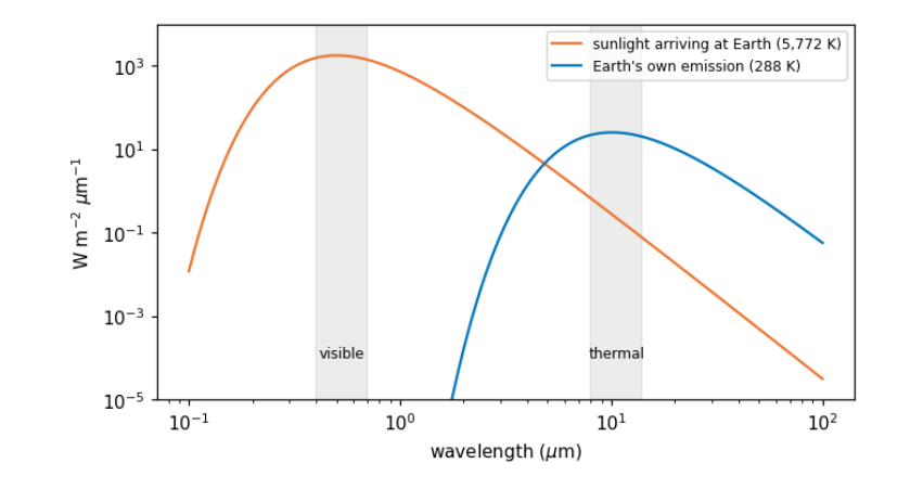
Sun: peak from the curve 0.50 um, Wien's law 0.50 um, total sigma*T^4 = 62,938,588 W/m2
Earth: peak from the curve 10.05 um, Wien's law 10.06 um, total sigma*T^4 = 390 W/m2
3.4 The atmosphere’s windows
Between the Sun, the ground and the satellite, light crosses the atmosphere twice. Gases absorb at particular wavelengths, because each molecule can only take up energy in steps that match its vibrations and rotations: water vapour absorbs strongly near 1.4, 1.9 and 2.7 \(\mu\)m and across much of the thermal infrared; carbon dioxide near 2.7, 4.3 and 15 \(\mu\)m; ozone absorbs ultraviolet. The ranges that pass are atmospheric windows, and satellite bands are placed inside them. Even inside windows, small particles and molecules scatter light, most strongly at short wavelengths (Rayleigh scattering goes as \(1/\lambda^4\)): the reason the sky is blue and why the blue band of any image looks hazy. Correcting for this is atmospheric correction, compared later in this notebook.
3.5 Bands and the four resolutions
A sensor records each band separately. Its design is a set of trade-offs, usually described as four resolutions:
-
spatial: the ground size of a pixel (Sentinel-2: 10, 20 or 60 m; Landsat: 30 m; MODIS: 250 to 1,000 m);
-
spectral: how many bands, and how narrow (Sentinel-2 has 13);
-
temporal: how often the same place is seen (Sentinel-2: every 5 days with two satellites; MODIS: daily);
-
radiometric: how finely brightness is divided (12 bits = 4,096 levels for Sentinel-2).
Finer pixels mean narrower swaths and fewer visits, so no sensor is best at all four. The catalogue describes each band; we read those descriptions directly.
catalog = pystac_client.Client.open("https://planetarycomputer.microsoft.com/api/stac/v1", modifier=planetary_computer.sign_inplace)
BBOX = [74.55, 36.25, 74.75, 36.40]                        # Hunza valley around Karimabad and Aliabad
items = sorted(catalog.search(collections=["sentinel-2-l2a"], bbox=BBOX, datetime="2025-03-01/2025-04-30",
                              query={"eo:cloud_cover": {"lt": 15}}).items(), key=lambda i: i.properties["eo:cloud_cover"])
item = items[0]
print("image:", item.id, "| date", item.properties["datetime"][:10], "| sun elevation",
      round(90 - item.properties["s2:mean_solar_zenith"], 1), "degrees")
rows = []
for key, a in item.assets.items():
    for b in a.extra_fields.get("eo:bands", []):
        rows.append(dict(asset=key, band=b.get("description", b["name"]), centre_um=b.get("center_wavelength"),
                         width_um=b.get("full_width_half_max"), pixel_m=a.extra_fields.get("gsd")))
bands = pd.DataFrame(rows).dropna(subset=["centre_um"]).sort_values("centre_um").reset_index(drop=True)
bands
image: S2B_MSIL2A_20250429T054639_R048_T43SDA_20250429T075112 | date 2025-04-29 | sun elevation 64.2 degrees
     asset                             band  centre_um  width_um  pixel_m
0      B01         Band 1 - Coastal aerosol      0.443     0.027       60
1      B02                    Band 2 - Blue      0.490     0.098       10
2   visual                    Band 2 - Blue      0.490     0.098       10
3      B03                   Band 3 - Green      0.560     0.045       10
4   visual                   Band 3 - Green      0.560     0.045       10
5   visual                     Band 4 - Red      0.665     0.038       10
6      B04                     Band 4 - Red      0.665     0.038       10
7      B05   Band 5 - Vegetation red edge 1      0.704     0.019       20
8      B06   Band 6 - Vegetation red edge 2      0.740     0.018       20
9      B07   Band 7 - Vegetation red edge 3      0.783     0.028       20
10     B08                     Band 8 - NIR      0.842     0.145       10
11     B8A  Band 8A - Vegetation red edge 4      0.865     0.033       20
12     B09             Band 9 - Water vapor      0.945     0.026       60
13     B11             Band 11 - SWIR (1.6)      1.610     0.143       20
14     B12             Band 12 - SWIR (2.2)      2.190     0.242       20
3.6 From digital numbers to reflectance
A file does not store "brightness" directly. It stores digital numbers (DNs): whole numbers, chosen so that the data fit in 16-bit integers and compress well. To get a physical quantity you apply the product's scale and offset:
For Sentinel-2 the quantification value is 10,000, and since processing baseline 04.00 (January 2022) the offset is -1,000, so that small negative values from the correction need not be cut off. Forgetting the offset makes every reflectance 0.1 too high: a classic, silent error. Reflectance is the fraction of incoming sunlight reflected, from 0 (absorbs everything) to 1 (reflects everything); fresh snow reaches about 0.9 in visible light.
DN 0 here means no data (outside the image), and must be masked before any statistics.
Reflectance above 1? The output below shows a few values above 1, which no real surface reflects. Level-2A images are corrected for terrain as well as for the atmosphere: the processor divides out how much sunlight each slope received, using a DEM. On steep slopes that received little sun, that division magnifies small errors and can overshoot. The terrain notebook checks this on the same image. Treat such values as artefacts of the correction and leave them out of statistics, or cap them, saying which you did.
def read(item, key, bbox, shape=None):
    with rasterio.open(item.assets[key].href) as src:
        win = from_bounds(*transform_bounds("EPSG:4326", src.crs, *bbox), src.transform)
        kw = dict(out_shape=shape, resampling=Resampling.bilinear) if shape else {}
        return src.read(1, window=win, **kw), src.profile

b04, prof = read(item, "B04", BBOX)
shape = b04.shape
dn = {b: read(item, b, BBOX, shape)[0] for b in ["B02", "B03", "B04", "B08", "B11", "B12"]}
baseline = float(item.properties["s2:processing_baseline"])
offset = -1000 if baseline >= 4.0 else 0
refl = {b: np.where(v == 0, np.nan, (v.astype("float32") + offset) / 10000) for b, v in dn.items()}
print("processing baseline", baseline, "-> offset", offset, "| data type in the file:", dn["B04"].dtype,
      "| grid:", shape, "pixels of", round(prof["transform"].a), "m")
print("red band, raw DN: min", int(dn["B04"][dn["B04"] > 0].min()), "max", int(dn["B04"].max()),
      "| reflectance: min", round(float(np.nanmin(refl["B04"])), 3), "max", round(float(np.nanmax(refl["B04"])), 3))
processing baseline 5.11 -> offset -1000 | data type in the file: uint16 | grid: (1670, 1801) pixels of 10 m
red band, raw DN: min 999 max 17148 | reflectance: min -0.0 max 1.615
3.7 Histograms and contrast
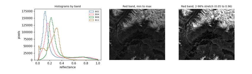
A histogram counts how many pixels have each value. It is the first thing to look at in any band: it shows the range, whether there are several kinds of surface (several peaks), and whether values pile up at the top (saturation, common over bright snow) or bottom.
Screens show 256 levels per colour, so to display a band you choose which values map to black and white. Using the minimum and maximum wastes the range on a few extreme pixels; a percentile stretch (here the 2nd to 98th percentile) maps most pixels across the full range. Stretching changes only the picture, never the data you analyse.
fig, ax = plt.subplots(1, 3, figsize=(11, 3.4))
for b, col in [("B02", "#4477aa"), ("B04", "#ee6677"), ("B08", "#228833"), ("B11", "#aa7733")]:
    ax[0].hist(refl[b][np.isfinite(refl[b])], bins=120, range=(0, 1.0), histtype="step", color=col, label=b)
ax[0].set_xlabel("reflectance")
ax[0].set_ylabel("pixels")
ax[0].legend(fontsize=7)
ax[0].set_title("Histograms by band", fontsize=9)
red = refl["B04"]
ax[1].imshow(red, cmap="gray", vmin=np.nanmin(red), vmax=np.nanmax(red))
ax[1].set_title("Red band, min to max", fontsize=9)
lo, hi = np.nanpercentile(red, [2, 98])
ax[2].imshow(red, cmap="gray", vmin=lo, vmax=hi)
ax[2].set_title(f"Red band, 2-98% stretch ({lo:.2f} to {hi:.2f})", fontsize=9)
for a in ax[1:]:
    a.set_axis_off()
plt.tight_layout()
plt.show()
3.8 Colour composites
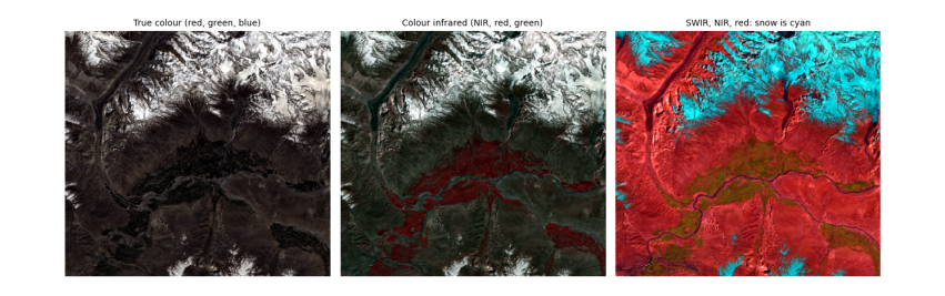
A colour picture is three bands shown as red, green and blue. True colour puts the red, green and blue bands in those places, as our eyes would see. False colour uses bands we cannot see. Two standard ones:
-
NIR, red, green (the "colour infrared" composite): healthy vegetation is bright red, because leaves reflect near infrared strongly. The reason is biological: inside a leaf, light scatters many times at the boundaries between water-filled cells and air spaces in the spongy mesophyll, and with no pigment absorbing in the near infrared, much of it comes back out. Chlorophyll, meanwhile, absorbs red and blue light for photosynthesis, so leaves are dark there.
-
SWIR, NIR, red: snow and ice turn cyan-blue and clouds stay white, because ice absorbs strongly in the shortwave infrared while cloud droplets, being small, still scatter it. This is how snow is told from cloud.
def stretch(a, p=(2, 98)):
    lo, hi = np.nanpercentile(a, p)
    return np.clip((a - lo) / (hi - lo), 0, 1)

def rgb(r, g, b):
    return np.dstack([stretch(refl[r]), stretch(refl[g]), stretch(refl[b])])

fig, ax = plt.subplots(1, 3, figsize=(12, 4.2))
for a, (r, g, b), title in zip(ax, [("B04", "B03", "B02"), ("B08", "B04", "B03"), ("B11", "B08", "B04")],
                               ["True colour (red, green, blue)", "Colour infrared (NIR, red, green)", "SWIR, NIR, red: snow is cyan"]):
    a.imshow(rgb(r, g, b))
    a.set_title(title, fontsize=9)
    a.set_axis_off()
plt.tight_layout()
plt.show()
3.9 Spectral signatures
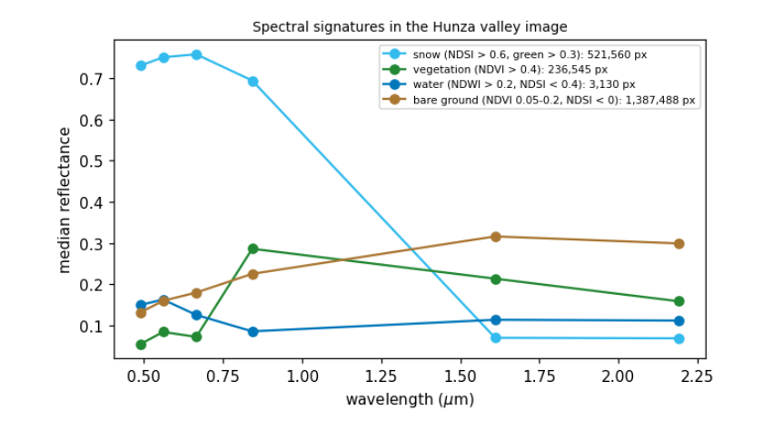
Plotting reflectance against wavelength for one kind of surface gives its spectral signature, the basis of every classification. Below we pick pixels by simple, stated rules and plot their median signatures. Each shape has a physical cause:
-
snow: very bright in visible and near infrared (ice crystals scatter), dark in SWIR (ice absorbs; the absorption grows with grain size, so old snow is darker in SWIR than fresh);
-
vegetation: low in blue and red (chlorophyll absorbs), a small green peak, a steep rise at about 0.7 \(\mu\)m (the red edge) to a high NIR plateau, then lower in SWIR where leaf water absorbs;
-
water: dark everywhere beyond green, because water absorbs near and shortwave infrared almost completely; a silty river is brighter in visible light from the suspended sediment;
-
bare rock and soil: rising gently with wavelength, with the details set by minerals (iron oxides absorb blue, clays and carbonates have SWIR absorption features).
ndsi = (refl["B03"] - refl["B11"]) / (refl["B03"] + refl["B11"])
ndvi = (refl["B08"] - refl["B04"]) / (refl["B08"] + refl["B04"])
ndwi = (refl["B03"] - refl["B08"]) / (refl["B03"] + refl["B08"])
rules = {"snow (NDSI > 0.6, green > 0.3)": (ndsi > 0.6) & (refl["B03"] > 0.3),
         "vegetation (NDVI > 0.4)": ndvi > 0.4,
         "water (NDWI > 0.2, NDSI < 0.4)": (ndwi > 0.2) & (ndsi < 0.4),
         "bare ground (NDVI 0.05-0.2, NDSI < 0)": (ndvi > 0.05) & (ndvi < 0.2) & (ndsi < 0)}
centre = dict(zip(bands.asset, bands.centre_um))
order = ["B02", "B03", "B04", "B08", "B11", "B12"]
fig, ax = plt.subplots(figsize=(7, 3.8))
for (name, m), col in zip(rules.items(), ["#33bbee", "#228833", "#0077bb", "#aa7733"]):
    med = [np.nanmedian(refl[b][m]) for b in order]
    ax.plot([centre[b] for b in order], med, "-o", color=col, label=f"{name}: {int(m.sum()):,} px")
ax.set_xlabel("wavelength ($\\mu$m)")
ax.set_ylabel("median reflectance")
ax.legend(fontsize=7)
ax.set_title("Spectral signatures in the Hunza valley image", fontsize=9)
plt.show()
3.10 What atmospheric correction changes
The image above is Level-2A: surface reflectance, after the Sen2Cor processor removed the effects of the atmosphere (scattering by air and aerosol, absorption by water vapour). The same scene also exists as Level-1C: top-of-atmosphere reflectance, what the satellite actually sees. Comparing the two shows what the atmosphere adds: a haze that lifts dark surfaces most in the blue band (Rayleigh scattering), and much less in the infrared.
Level-1C files on Amazon are in a "requester pays" bucket (reading them needs a paid AWS account), so this comparison uses Google Earth Engine, which holds both levels of the same image (see the data access notebook for setting it up). The pixels are chosen by the same water and vegetation rules, applied to the surface image.
import os
from pathlib import Path
EE_PROJECT = os.environ.get("EE_PROJECT")
if EE_PROJECT and (Path.home() / ".config" / "earthengine" / "credentials").exists():
    import ee
    ee.Initialize(project=EE_PROJECT)
    region = ee.Geometry.Rectangle(BBOX)
    pid = item.properties["s2:product_uri"].replace(".SAFE", "") if "s2:product_uri" in item.properties else None
    day = ee.Date(item.properties["datetime"][:10])
    pick = lambda c: ee.Image(ee.ImageCollection(c).filterBounds(region).filterDate(day, day.advance(1, "day")).first())
    sr, toa_img = pick("COPERNICUS/S2_SR_HARMONIZED"), pick("COPERNICUS/S2_HARMONIZED")
    s = sr.divide(10000)       # Earth Engine's harmonized collections have the -1000 offset already removed
    water_m = s.normalizedDifference(["B3", "B8"]).gt(0.2).And(s.normalizedDifference(["B3", "B11"]).lt(0.4))
    veg_m = s.normalizedDifference(["B8", "B4"]).gt(0.4)
    out = {}
    for label, m in [("water", water_m), ("vegetation", veg_m)]:
        for level, img in [("top of atmosphere", toa_img), ("surface", sr)]:
            v = img.select(["B2", "B4", "B8", "B11"]).divide(10000).updateMask(m).reduceRegion(ee.Reducer.median(), region, 20, maxPixels=1e9).getInfo()
            out[f"{label}, {level}"] = v
    tab = pd.DataFrame(out).T.rename(columns={"B2": "blue", "B4": "red", "B8": "NIR", "B11": "SWIR"})[["blue", "red", "NIR", "SWIR"]].round(3)
    print(tab.to_string())
else:
    print("Earth Engine not set up here: see the data access notebook. The comparison is skipped.")
blue    red    NIR   SWIR
water, top of atmosphere       0.161  0.126  0.095  0.099
water, surface                 0.143  0.116  0.080  0.101
vegetation, top of atmosphere  0.104  0.087  0.253  0.188
vegetation, surface            0.057  0.074  0.287  0.212
Reading the table: over vegetation, which is dark in blue, the top-of-atmosphere blue value is almost twice the surface value: about half of what the satellite records there is light scattered by the air itself (Rayleigh scattering, strongest at short wavelengths), which the correction removes. In the near infrared the correction works the other way, raising the value, because it restores light that aerosol and water vapour absorbed on the way. The river here is silty and bright, so the haze makes up a smaller share of its signal and its values change less. This is why indices and classifications should use surface reflectance when it exists, and why comparing images from different dates without correction mixes changes in the atmosphere with changes on the ground.
3.11 What to remember
-
A pixel value is light: reflected sunlight in visible and shortwave bands, emitted heat in thermal bands.
-
Planck's and Wien's laws explain which; atmospheric windows explain where bands sit.
-
Convert DNs to physical units with the product's scale and offset, and mask the no-data and coded values.
-
Look at histograms first; stretch only for display.
-
Surfaces differ for physical, chemical and biological reasons, and those reasons explain every index.
Exercises. (1) Compute the photon energy at 0.665 \(\mu\)m and compare it with the energy needed to break a typical chemical bond (about \(5 \times 10^{-19}\) J). (2) Find the date with the most snow in the same valley in autumn and compare signatures of fresh and old snow in B11. (3) Repeat the atmospheric comparison for a hazy summer date.
4. Preparing images
4.1 Overview
Raw images rarely line up with each other or with your study area. Before any analysis they are pre-processed: put on a common map grid, cut to the area, joined where an area spans several images, stacked into one array, cleaned of cloud and missing data, and combined over time into a composite. Each step changes the numbers a little, and each has a right and a wrong way. This notebook does them all on Sentinel-2 images of the upper Hunza valley.
What you will learn: coordinate reference systems and map projections; how a raster is placed on the Earth (the transform); clipping to a box and to a polygon; reprojection and the choice of resampling; mosaicking two tiles; stacking bands of different pixel sizes; masking no-data and cloud with the scene classification; and building a median composite from many dates.
import importlib.util, subprocess, sys
need = {"pystac_client": "pystac-client", "planetary_computer": "planetary-computer", "rasterio": "rasterio", "geopandas": "geopandas"}
missing = [p for m, p in need.items() if importlib.util.find_spec(m) is None]
if missing:
    subprocess.run([sys.executable, "-m", "pip", "install", "-q", *missing], check=True)
import numpy as np
import pandas as pd
import geopandas as gpd
import matplotlib.pyplot as plt
import rasterio
from rasterio.windows import from_bounds
from rasterio.warp import transform_bounds, reproject, calculate_default_transform, Resampling
from rasterio.merge import merge
from rasterio.mask import mask as rio_mask
from shapely.geometry import box, Polygon
import pystac_client, planetary_computer
plt.rcParams.update({"figure.dpi": 110})
catalog = pystac_client.Client.open("https://planetarycomputer.microsoft.com/api/stac/v1", modifier=planetary_computer.sign_inplace)
4.2 Coordinates, projections and the transform
The Earth is close to an ellipsoid, a sphere slightly flattened at the poles (equatorial radius 6,378.137 km, polar 6,356.752 km in the WGS84 model). A position on it is given by latitude and longitude in degrees. Maps and images are flat, so every flat map uses a projection: a formula from (latitude, longitude) to (x, y) in metres. No projection keeps every property; each preserves some (areas, angles or distances) and distorts others.
Sentinel-2 and Landsat use UTM (Universal Transverse Mercator): the globe is cut into 60 zones 6 degrees wide, each with its own projection that is accurate to within 0.04% inside the zone. Hunza lies in zone 43 north (EPSG:32643). A CRS (coordinate reference system) names the ellipsoid and projection; an EPSG code is the standard number for one.
A raster is placed on the map by its affine transform, six numbers that map a pixel's (column, row) to (x, y):
where \(a\) is the pixel width, \(e\) the pixel height (negative, because rows count downwards), \(c, f\) the coordinates of the top-left corner, and \(b, d\) are zero unless the image is rotated.
items = sorted(catalog.search(collections=["sentinel-2-l2a"], bbox=[74.4, 36.3, 74.9, 36.6], datetime="2024-06-01/2024-09-30",
                              query={"eo:cloud_cover": {"lt": 60}}).items(), key=lambda i: i.properties["datetime"])
print(len(items), "summer 2024 images; tiles:", sorted({i.properties["s2:mgrs_tile"] for i in items}))
item = min(items, key=lambda i: i.properties["eo:cloud_cover"])
with rasterio.open(item.assets["B04"].href) as src:
    print("CRS:", src.crs, "| size:", src.width, "x", src.height, "| pixel:", src.res)
    print("transform:", tuple(round(v, 1) for v in src.transform[:6]))
    col, row = 5000, 5000
    x, y = src.transform * (col, row)
    lon, lat = rasterio.warp.transform(src.crs, "EPSG:4326", [x], [y])
    print(f"pixel (col {col}, row {row}) -> x {x:,.0f} m, y {y:,.0f} m -> {lat[0]:.4f} N, {lon[0]:.4f} E")
15 summer 2024 images; tiles: ['43SDA']
CRS: EPSG:32643 | size: 10980 x 10980 | pixel: (10.0, 10.0)
transform: (10.0, 0.0, 399960.0, 0.0, -10.0, 4100040.0)
pixel (col 5000, row 5000) -> x 449,960 m, y 4,050,040 m -> 36.5945 N, 74.4406 E
4.3 Clipping: a box, then a polygon
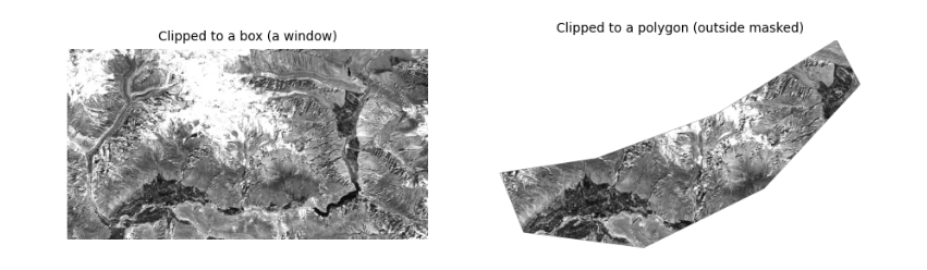
Clipping keeps only your area. With a box, the fastest way is to read just the window of rows and columns that covers it (the file is never read in full). With an irregular area (a catchment, a district) you then mask the pixels outside the polygon. The polygon must be in the same CRS as the raster: convert it first.
The polygon here is drawn by hand around the valley floor between Aliabad and Gulmit, as an example of a study area.
AOI = [74.55, 36.28, 74.95, 36.45]
valley = gpd.GeoDataFrame(geometry=[Polygon([(74.60, 36.30), (74.70, 36.29), (74.80, 36.33), (74.88, 36.40),
                                             (74.86, 36.43), (74.76, 36.38), (74.66, 36.35), (74.58, 36.34)])], crs="EPSG:4326")
with rasterio.open(item.assets["B04"].href) as src:
    win = from_bounds(*transform_bounds("EPSG:4326", src.crs, *AOI), src.transform)
    red = src.read(1, window=win)
    wtf = src.window_transform(win)
    poly = valley.to_crs(src.crs)
    clipped, ctf = rio_mask(src, poly.geometry, crop=True, nodata=0)
print("box window:", red.shape, "| polygon clip:", clipped.shape[1:], "| pixels inside polygon:", int((clipped[0] > 0).sum()))
fig, ax = plt.subplots(1, 2, figsize=(10, 3.6))
ax[0].imshow(red, cmap="gray", vmin=1000, vmax=4000)
ax[0].set_title("Clipped to a box (a window)", fontsize=9)
ax[1].imshow(np.ma.masked_equal(clipped[0], 0), cmap="gray", vmin=1000, vmax=4000)
ax[1].set_title("Clipped to a polygon (outside masked)", fontsize=9)
for a in ax:
    a.set_axis_off()
plt.show()
box window: (1895, 3593) | polygon clip: (1551, 2694) | pixels inside polygon: 1672083
4.4 Reprojection and resampling
To combine data on different grids (a 10 m UTM image and a 30 m DEM in degrees, say) one must be reprojected onto the other's grid. Each new pixel takes its value from the old pixels near its centre, by a resampling rule:
-
nearest neighbour: the closest old pixel. Keeps original values exactly; the only correct choice for categories (land cover classes, masks, quality flags), which must never be averaged.
-
bilinear: a distance-weighted mean of the 4 nearest pixels. Smooth; good for continuous values (reflectance, elevation, temperature).
-
cubic: uses 16 pixels; sharper, but can overshoot past the original range.
-
average: the mean of all old pixels inside each new one; the right choice when making pixels much larger.
Below, the red band is reprojected to geographic coordinates (EPSG:4326) at about 30 m, with each rule, and we compare the statistics. Averaging changes extremes most: bright and dark single pixels are smoothed away.
dst_crs = "EPSG:4326"
tf, w, h = calculate_default_transform(src.crs, dst_crs, red.shape[1], red.shape[0], *rasterio.transform.array_bounds(*red.shape, wtf), resolution=0.0003)
rows = []
for rule in [Resampling.nearest, Resampling.bilinear, Resampling.cubic, Resampling.average]:
    out = np.zeros((h, w), "float32")
    reproject(red.astype("float32"), out, src_transform=wtf, src_crs=src.crs, dst_transform=tf, dst_crs=dst_crs,
              resampling=rule, src_nodata=0, dst_nodata=0)
    v = out[out > 0]
    rows.append(dict(rule=rule.name, pixels=v.size, mean=v.mean(), min=v.min(), max=v.max(), std=v.std()))
v = red[red > 0]
rows.insert(0, dict(rule="original 10 m", pixels=v.size, mean=v.mean(), min=v.min(), max=v.max(), std=v.std()))
pd.DataFrame(rows).round(1)
rule   pixels    mean          min           max     std
0  original 10 m  6808735  3214.9   437.000000  16753.000000  2089.7
1        nearest   760593  3214.9  1012.000000  16751.000000  2090.2
2       bilinear   760593  3215.4  1039.599976  16621.699219  1999.1
3          cubic   760593  3215.4   974.000000  17851.199219  2036.2
4        average   761906  3216.2  1038.400024  16703.900391  2024.4
4.5 Mosaicking: joining tiles
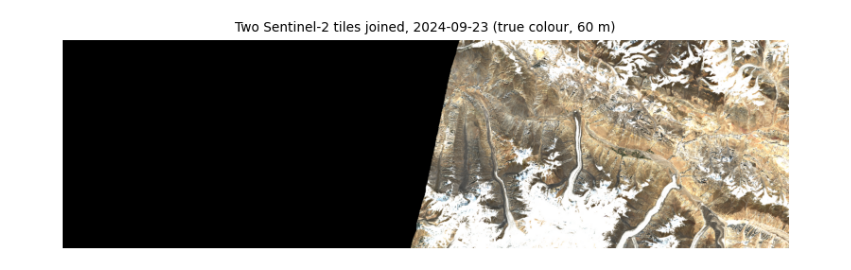
Sentinel-2 is cut into 110 by 110 km tiles on the MGRS grid; Landsat into path/row scenes. An area across a tile boundary needs a mosaic. Tiles from the same orbit and date line up exactly (same sun, same atmosphere); tiles from different dates show seams. Where tiles overlap, a rule decides which value wins: the first tile, the last, or the mean. Here we join two tiles from the same orbit and day.
WIDE = [74.3, 36.3, 75.6, 36.6]                          # wider than one tile: reaches the next tile east
wide_items = catalog.search(collections=["sentinel-2-l2a"], bbox=WIDE, datetime="2024-06-01/2024-09-30",
                            query={"eo:cloud_cover": {"lt": 20}}).items()
by_tile = {}
for i in wide_items:
    by_tile.setdefault(i.properties["datetime"][:10], {})[i.properties["s2:mgrs_tile"]] = i
day, tiles = next((d, t) for d, t in sorted(by_tile.items(), key=lambda kv: -len(kv[1])) if len(t) >= 2)
print("date with", len(tiles), "tiles:", day, sorted(tiles))
srcs = [rasterio.open(t.assets["visual"].href) for t in list(tiles.values())[:2]]
bounds = transform_bounds("EPSG:4326", srcs[0].crs, *WIDE)
mosaic, mtf = merge(srcs, bounds=bounds, res=60, resampling=Resampling.average, method="first", nodata=0)
for s in srcs:
    s.close()
print("mosaic:", mosaic.shape, "(bands, rows, columns) at 60 m")
plt.figure(figsize=(9, 3.2))
plt.imshow(np.moveaxis(mosaic, 0, -1))
plt.title(f"Two Sentinel-2 tiles joined, {day} (true colour, 60 m)", fontsize=9)
plt.axis("off")
plt.show()
date with 2 tiles: 2024-09-23 ['43SDA', '43SEA']
mosaic: (3, 558, 1945) (bands, rows, columns) at 60 m
4.6 Stacking bands of different pixel sizes
Analysis is easiest with all bands in one 3-D array (band, row, column) on one grid. Sentinel-2's bands come at 10, 20 and 60 m, so the 20 m bands are resampled to 10 m (bilinear, since reflectance is continuous) and the 20 m scene classification layer (SCL), which holds categories, with nearest neighbour.
STUDY = [74.60, 36.30, 74.80, 36.42]
def read_to(item, key, bbox, shape, rule):
    with rasterio.open(item.assets[key].href) as s:
        win = from_bounds(*transform_bounds("EPSG:4326", s.crs, *bbox), s.transform)
        return s.read(1, window=win, out_shape=shape, resampling=rule)

with rasterio.open(item.assets["B02"].href) as s:
    win = from_bounds(*transform_bounds("EPSG:4326", s.crs, *STUDY), s.transform)
    shape = s.read(1, window=win).shape
keys = ["B02", "B03", "B04", "B08", "B11", "B12"]
stack = np.stack([read_to(item, k, STUDY, shape, Resampling.bilinear) for k in keys])
scl = read_to(item, "SCL", STUDY, shape, Resampling.nearest)
print("stack:", stack.shape, stack.dtype, "| SCL:", scl.shape, "| SCL classes present:", sorted(np.unique(scl).tolist()))
stack: (6, 1337, 1798) uint16 | SCL: (1337, 1798) | SCL classes present: [2, 3, 4, 5, 6, 7, 8, 9, 11]
4.7 Masking no-data and cloud
Two kinds of pixel must be removed before statistics. No-data pixels (outside the image, value 0 here) carry no measurement. Cloud and cloud shadow hide the ground. Sentinel-2 Level-2A includes the scene classification layer, a per-pixel label from the Sen2Cor processor:
| SCL | Meaning | SCL | Meaning |
|---|---|---|---|
| no data | 6 | water | |
| 1 | saturated or defective | 7 | unclassified |
| 2 | dark area | 8 | cloud, medium probability |
| 3 | cloud shadow | 9 | cloud, high probability |
| 4 | vegetation | 10 | thin cirrus |
| 5 | not vegetated | 11 | snow or ice |
A mask is a true/false array; numpy's where replaces masked values with NaN ("not a number"), which statistics functions such as nanmean skip. Masks are never perfect: SCL confuses bright snow with cloud and dark shadows with water, especially in mountains, so always look at what you remove. In the output below about a sixth of the valley is "dark area": mostly slopes in the shadow of mountains, which the mask keeps, since they are real ground; their values are low because little sunlight reaches them, the topographic effect again.
names = {0: "no data", 1: "saturated", 2: "dark area", 3: "cloud shadow", 4: "vegetation", 5: "not vegetated", 6: "water",
         7: "unclassified", 8: "cloud medium", 9: "cloud high", 10: "cirrus", 11: "snow or ice"}
v, n = np.unique(scl, return_counts=True)
print(pd.Series(n / n.sum() * 100, index=[names[int(x)] for x in v]).round(1).to_string(), "\n(% of pixels)")
bad = np.isin(scl, [0, 1, 3, 8, 9, 10])
refl = np.where(bad[None], np.nan, (stack.astype("float32") - 1000) / 10000)
print("kept", f"{100 * (~bad).mean():.1f}% of pixels")
dark area        16.5
cloud shadow      0.0
vegetation        7.7
not vegetated    52.4
water             0.3
unclassified      0.3
cloud medium      0.1
cloud high        0.0
snow or ice      22.6
(% of pixels)
kept 99.9% of pixels
4.8 Composites over time
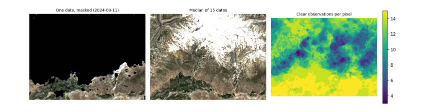
One image is one moment, often with cloud. A composite combines many dates into one cloud-free picture by taking, at each pixel, a statistic over the clear observations. The median is the usual choice: it ignores the few cloudy or shadowed values that slip past the mask, which a mean would not. The cost is that a composite no longer shows one moment, so it suits slowly changing things (land cover) better than quick ones (snow on a given day).
Below, every summer 2024 image of the study area is masked and the median taken. We use the 20 m bands to keep memory low.
use = [i for i in items if i.properties["s2:mgrs_tile"] == item.properties["s2:mgrs_tile"]]
with rasterio.open(item.assets["B11"].href) as s:
    win = from_bounds(*transform_bounds("EPSG:4326", s.crs, *STUDY), s.transform)
    shape20 = s.read(1, window=win).shape
layers, clear = [], []
for it in use:
    s_cl = read_to(it, "SCL", STUDY, shape20, Resampling.nearest)
    ok = ~np.isin(s_cl, [0, 1, 3, 8, 9, 10])
    off = -1000 if float(it.properties["s2:processing_baseline"]) >= 4 else 0
    rgb = np.stack([read_to(it, k, STUDY, shape20, Resampling.average) for k in ["B04", "B03", "B02"]]).astype("float32")
    layers.append(np.where(ok[None], (rgb + off) / 10000, np.nan))
    clear.append(round(float(ok.mean()), 2))
cube = np.stack(layers)                                   # date, band, row, column
median = np.nanmedian(cube, axis=0)
count = np.isfinite(cube[:, 0]).sum(0)
print(len(use), "dates; clear share per date:", clear)
print("clear observations per pixel: min", int(count.min()), "median", int(np.median(count)), "max", int(count.max()))
fig, ax = plt.subplots(1, 3, figsize=(12, 3.6))
show = lambda a: np.clip(np.moveaxis(a, 0, -1) / 0.35, 0, 1)
worst = int(np.argmin(clear))
ax[0].imshow(show(np.nan_to_num(cube[worst], nan=0)))
ax[0].set_title(f"One date, masked ({use[worst].properties['datetime'][:10]})", fontsize=9)
ax[1].imshow(show(np.nan_to_num(median, nan=0)))
ax[1].set_title(f"Median of {len(use)} dates", fontsize=9)
im = ax[2].imshow(count, cmap="viridis")
ax[2].set_title("Clear observations per pixel", fontsize=9)
plt.colorbar(im, ax=ax[2], fraction=0.04)
for a in ax:
    a.set_axis_off()
plt.tight_layout()
plt.show()
15 dates; clear share per date: [0.78, 0.6, 0.64, 0.95, 0.88, 0.95, 1.0, 0.71, 0.82, 0.83, 0.46, 0.88, 0.27, 1.0, 0.72]
clear observations per pixel: min 3 median 12 max 15
4.9 Saving the result properly
A result is only useful if others can open it in any GIS and know what it is. Save rasters as Cloud-Optimised GeoTIFF with the CRS and transform, a no-data value, compression, band descriptions, and a few words of metadata on how it was made. (Reading it back reports the driver as GTiff: a COG is an ordinary GeoTIFF with its internal tiles and overviews arranged for reading over the web.)
with rasterio.open(item.assets["B11"].href) as s:
    crs20, tf20 = s.crs, rasterio.windows.transform(win, s.transform)
profile = dict(driver="COG", dtype="float32", count=3, width=shape20[1], height=shape20[0], crs=crs20,
               transform=tf20, nodata=np.nan, compress="deflate")
with rasterio.open("hunza_median_summer2024.tif", "w", **profile) as dst:
    dst.write(median.astype("float32"))
    for k, name in enumerate(["red", "green", "blue"], 1):
        dst.set_band_description(k, f"{name} surface reflectance")
    dst.update_tags(source="Sentinel-2 L2A via Microsoft Planetary Computer", method=f"per-pixel median of {len(use)} dates, SCL cloud mask",
                    period="2024-06-01/2024-09-30")
with rasterio.open("hunza_median_summer2024.tif") as chk:
    print(chk.profile["driver"], chk.crs, chk.res, chk.count, "bands |", chk.descriptions, "|", chk.tags()["method"])
GTiff EPSG:32643 (20.0, 20.0) 3 bands | ('red surface reflectance', 'green surface reflectance', 'blue surface reflectance') | per-pixel median of 15 dates, SCL cloud mask
4.10 What to remember
-
Know your CRS, and convert vectors to the raster's CRS, not the other way round, unless you mean to resample.
-
Read only the window you need; clip to polygons after.
-
Nearest neighbour for categories, bilinear or average for continuous values.
-
Mask no-data and cloud before any statistic, and look at what the mask removed.
-
A median composite gives a clear picture of a season, at the cost of losing the moment.
-
Save with CRS, no-data, descriptions and a record of how the file was made.
Exercises. (1) Repeat the composite with the mean instead of the median and find where they differ most. (2) Reproject the composite to UTM zone 43 at 30 m with each resampling rule and compare. (3) Draw a polygon around your own study area and compute the share of clear observations inside it per month.
5. Terrain
5.1 Overview
In mountains, the shape of the ground controls almost everything a satellite sees: how much sunlight a slope gets, how cold it is, where snow lasts, where water flows. A digital elevation model (DEM) describes that shape, and from it come slope, aspect, shading and corrections. This notebook works with the Copernicus 30 m DEM over the Hunza valley, where the ground rises from about 2,000 m at the river to over 7,000 m on Rakaposhi and Ultar within 15 km.
What you will learn: how DEMs are made and what their heights mean; slope and aspect from finite differences; hillshade; how the angle between sun and slope sets illumination; topographic correction of an image; elevation bands and hypsometry; valley profiles and the geology behind them; and lapse rates.
import importlib.util, subprocess, sys
need = {"pystac_client": "pystac-client", "planetary_computer": "planetary-computer", "rasterio": "rasterio"}
missing = [p for m, p in need.items() if importlib.util.find_spec(m) is None]
if missing:
    subprocess.run([sys.executable, "-m", "pip", "install", "-q", *missing], check=True)
import numpy as np
import pandas as pd
import matplotlib.pyplot as plt
import rasterio
from rasterio.windows import from_bounds
from rasterio.warp import transform_bounds, reproject, Resampling
from rasterio.merge import merge
import pystac_client, planetary_computer
plt.rcParams.update({"figure.dpi": 110})
catalog = pystac_client.Client.open("https://planetarycomputer.microsoft.com/api/stac/v1", modifier=planetary_computer.sign_inplace)
BBOX = [74.55, 36.25, 74.75, 36.40]
5.2 What a DEM is
A DEM is a raster whose values are heights. Two kinds matter:
-
a digital surface model (DSM) gives the height of whatever the sensor first hits: tree tops, roofs, ice;
-
a digital terrain model (DTM) gives the bare ground, with vegetation and buildings removed.
Global DEMs are made by measuring the same ground from two viewpoints. SRTM (2000) and Copernicus DEM (from the TanDEM-X mission, 2011-2015) use radar interferometry: two radar antennas a known distance apart receive the echo from each point, and the tiny difference in the travel time (seen as a phase difference of the radar wave) gives the height by trigonometry. ASTER and ALOS DEMs use optical stereo: two images from different angles, as our two eyes judge depth. Copernicus GLO-30 is a DSM at 30 m with a typical vertical error of a few metres, larger on steep slopes and in radar shadow.
What "height" means. Heights need a zero. GPS measures height above the ellipsoid; maps use height above the geoid, the surface the sea would take if it extended under the land, which follows the pull of gravity and differs from the ellipsoid by up to 100 m (in this region the geoid is about 30 m below it). Copernicus DEM heights are above the EGM2008 geoid, so they match "metres above sea level" on maps.
dems = list(catalog.search(collections=["cop-dem-glo-30"], bbox=BBOX).items())
print("DEM tiles covering the area:", [d.id for d in dems])
srcs = [rasterio.open(d.assets["data"].href) for d in dems]
dem, dtf = merge(srcs, bounds=BBOX)
crs = srcs[0].crs
for s in srcs:
    s.close()
dem = dem[0].astype("float64")
print("CRS:", crs, "| pixel:", round(dtf.a * 3600, 2), "x", round(-dtf.e * 3600, 2), "arc-seconds | grid:", dem.shape)
print(f"height range {dem.min():,.0f} to {dem.max():,.0f} m; relief {dem.max() - dem.min():,.0f} m in a {abs(BBOX[2]-BBOX[0])*111*np.cos(np.radians(36.3)):.0f} km wide box")
DEM tiles covering the area: ['Copernicus_DSM_COG_10_N36_00_E074_00_DEM']
CRS: EPSG:4326 | pixel: 1.0 x 1.0 arc-seconds | grid: (540, 720)
height range 1,930 to 7,302 m; relief 5,371 m in a 18 km wide box
5.3 Slope and aspect
Slope is how steep the ground is; aspect is the compass direction it faces. Both come from the rate of change of height in the east-west and north-south directions, \(\partial z/\partial x\) and \(\partial z/\partial y\). On a grid these derivatives are estimated by finite differences: the difference between neighbours divided by their distance. Horn's method (1981), used by most GIS software, weights the eight neighbours of each cell:
with cells numbered 1-9 from top left. Then
measured clockwise from north. One trap: this DEM's pixels are in degrees, so \(\Delta x\) and \(\Delta y\) must be converted to metres first. A degree of latitude is about 111.3 km everywhere, but a degree of longitude shrinks with \(\cos(\text{latitude})\): at 36.3 N it is only about 89.7 km.
lat0 = np.radians((BBOX[1] + BBOX[3]) / 2)
dx = dtf.a * 111320 * np.cos(lat0)                 # metres per pixel east-west
dy = -dtf.e * 110950                               # metres per pixel north-south (a degree of latitude near 36 N)
def horn(dem, dx, dy):
    """Slope and aspect (degrees) by Horn's method; dx, dy are pixel sizes in metres; rows run north to south."""
    z = np.pad(dem, 1, mode="edge")
    z1, z2, z3 = z[:-2, :-2], z[:-2, 1:-1], z[:-2, 2:]
    z4, z6 = z[1:-1, :-2], z[1:-1, 2:]
    z7, z8, z9 = z[2:, :-2], z[2:, 1:-1], z[2:, 2:]
    dzdx = ((z3 + 2 * z6 + z9) - (z1 + 2 * z4 + z7)) / (8 * dx)
    dzdy = ((z7 + 2 * z8 + z9) - (z1 + 2 * z2 + z3)) / (8 * dy)  # positive when height increases southwards
    slope = np.degrees(np.arctan(np.hypot(dzdx, dzdy)))
    aspect = (np.degrees(np.arctan2(-dzdx, dzdy)) + 360) % 360  # direction the slope faces, 0 = north, 90 = east
    return slope, aspect

slope, aspect = horn(dem, dx, dy)
print(f"pixel size: {dx:.1f} m east-west, {dy:.1f} m north-south")
print(f"slope: median {np.median(slope):.0f} deg, 90th percentile {np.percentile(slope, 90):.0f} deg, steepest {slope.max():.0f} deg")
#### a check on surfaces whose answer we know: a plane rising 1 m per metre eastwards has slope 45 deg and faces west (270);
#### one rising southwards faces north (0)
xx = np.arange(7)[None, :].repeat(7, 0) * 30.0
for name, surf in [("rising east", xx), ("rising south", xx.T)]:
    s_, a_ = horn(surf, 30.0, 30.0)
    print(f"known-answer test, plane {name}: slope {s_[3, 3]:.1f} deg, aspect {a_[3, 3]:.0f} deg")
pixel size: 24.9 m east-west, 30.8 m north-south
slope: median 38 deg, 90th percentile 55 deg, steepest 81 deg
known-answer test, plane rising east: slope 45.0 deg, aspect 270 deg
known-answer test, plane rising south: slope 45.0 deg, aspect 0 deg
5.4 Hillshade: how the Sun lights the slopes
The brightness of a slope in sunlight depends on the angle \(i\) between the Sun's rays and the perpendicular to the slope (the incidence angle). For a sun at zenith angle \(\theta_z\) (angle from straight up) and azimuth \(\phi_s\), and a slope \(s\) facing \(a\), spherical trigonometry gives
A slope facing the sun has \(\cos i\) near 1, a slope facing away near 0 or negative (in shadow). A hillshade is just \(\cos i\) drawn in grey, with an imagined sun usually from the north-west at 45 degrees, because our eyes read relief best when light comes from the top of the picture.
def cos_incidence(slope_deg, aspect_deg, sun_zenith, sun_azimuth):
    s, a = np.radians(slope_deg), np.radians(aspect_deg)
    tz, ps = np.radians(sun_zenith), np.radians(sun_azimuth)
    return np.cos(tz) * np.cos(s) + np.sin(tz) * np.sin(s) * np.cos(ps - a)

hill = cos_incidence(slope, aspect, 45, 315)
fig, ax = plt.subplots(1, 3, figsize=(12, 3.6))
im0 = ax[0].imshow(dem, cmap="terrain")
plt.colorbar(im0, ax=ax[0], fraction=0.04, label="m")
ax[0].set_title("Elevation", fontsize=9)
im1 = ax[1].imshow(slope, cmap="magma_r", vmax=60)
plt.colorbar(im1, ax=ax[1], fraction=0.04, label="degrees")
ax[1].set_title("Slope", fontsize=9)
ax[2].imshow(hill, cmap="gray", vmin=0, vmax=1)
ax[2].set_title("Hillshade (sun from NW, 45 deg up)", fontsize=9)
for a in ax:
    a.set_axis_off()
plt.tight_layout()
plt.show()
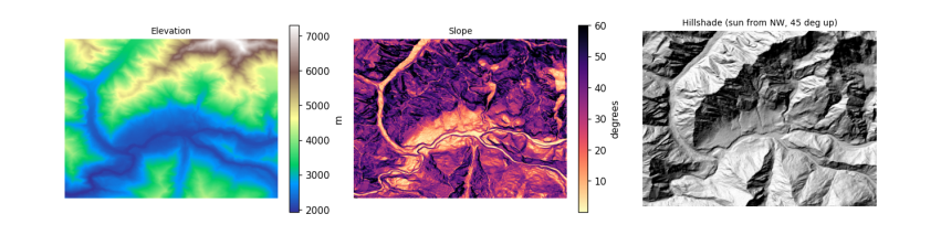
5.5 Topographic correction
With the real sun position at the moment an image was taken, \(\cos i\) says how much more or less light each slope received than flat ground. The simplest cosine correction divides that out: \(\rho_{flat} = \rho \cdot \cos\theta_z / \cos i\). It over-corrects slopes facing away from the sun, because those still receive light scattered from the sky and from neighbouring slopes. The C-correction (Teillet et al. 1982) fixes that with a constant \(c\) estimated from the image itself: regress reflectance on \(\cos i\) (\(\rho = m \cos i + b\)), set \(c = b/m\), and use
A good correction removes the relationship between brightness and illumination: afterwards, sunlit and shaded slopes of the same surface look alike. So the first question to ask of any image is whether that relationship is there at all. We check the Sentinel-2 Level-2A image from the physics notebook, on its own UTM grid with the DEM reprojected onto it.
item = sorted(catalog.search(collections=["sentinel-2-l2a"], bbox=BBOX, datetime="2025-03-01/2025-04-30",
                             query={"eo:cloud_cover": {"lt": 15}}).items(), key=lambda i: i.properties["eo:cloud_cover"])[0]
sz, sa = item.properties["s2:mean_solar_zenith"], item.properties["s2:mean_solar_azimuth"]
print(item.id[:38], "| sun zenith", round(sz, 1), "| sun azimuth", round(sa, 1))
#### Everything goes on the image's own grid (UTM, 30 m, averaging the 10 m pixels); the DEM is reprojected onto it with
#### bilinear resampling, since heights are continuous, and slope is then computed in metres directly.
with rasterio.open(item.assets["B04"].href) as src:
    win = from_bounds(*transform_bounds("EPSG:4326", src.crs, *BBOX), src.transform)
    shape30 = (int(win.height // 3), int(win.width // 3))
    red = src.read(1, window=win, out_shape=shape30, resampling=Resampling.average).astype("float64")
    utm, tf30 = src.crs, src.window_transform(win) * rasterio.Affine.scale(win.width / shape30[1], win.height / shape30[0])
with rasterio.open(item.assets["SCL"].href) as s:
    scl = s.read(1, window=from_bounds(*transform_bounds("EPSG:4326", s.crs, *BBOX), s.transform), out_shape=shape30,
                 resampling=Resampling.nearest)
dem_utm = np.zeros(shape30)
reproject(dem, dem_utm, src_transform=dtf, src_crs=crs, dst_transform=tf30, dst_crs=utm, resampling=Resampling.bilinear)
slope_u, aspect_u = horn(dem_utm, tf30.a, -tf30.e)
red = np.where(red == 0, np.nan, (red - 1000) / 10000)
cosi = cos_incidence(slope_u, aspect_u, sz, sa)
snow = (scl == 11) & np.isfinite(red) & (cosi > 0.05)
print(f"snow pixels: {snow.sum():,}; correlation of red reflectance with cos i: {np.corrcoef(cosi[snow], red[snow])[0, 1]:.3f}")
hi = snow & (red > 1)
print(f"pixels above 1: {hi.sum():,}; their median cos i {np.median(cosi[hi]):.2f} (all snow {np.median(cosi[snow]):.2f}),",
      f"median slope {np.median(slope_u[hi]):.0f} deg (all snow {np.median(slope_u[snow]):.0f})")
S2B_MSIL2A_20250429T054639_R048_T43SDA | sun zenith 25.8 | sun azimuth 144.6
snow pixels: 92,855; correlation of red reflectance with cos i: -0.034
pixels above 1: 3,743; their median cos i 0.53 (all snow 0.76), median slope 45 deg (all snow 43)
There is no relationship left to correct. The Level-2A processor (Sen2Cor) already applies a terrain correction with a DEM as part of its atmospheric correction, so brightness no longer depends on illumination. The few values above 1 sit on slopes that received much less sun than typical snow (and are slightly steeper): where \(\cos i\) is small, dividing by it magnifies small errors in the DEM or the sun geometry, so a correction can overshoot. Checking for the relationship before correcting is what stops anyone correcting the same image twice.
The uncorrected Level-1C (top-of-atmosphere) image still contains the effect. Its files on Amazon are in a "requester pays" bucket, so the cell below uses Google Earth Engine (see the data access notebook), which computes slope and aspect from the same Copernicus DEM, fits the C-correction to snow pixels, and compares the correlation before and after.
import os
from pathlib import Path
EE_PROJECT = os.environ.get("EE_PROJECT")
if EE_PROJECT and (Path.home() / ".config" / "earthengine" / "credentials").exists():
    import ee
    ee.Initialize(project=EE_PROJECT)
    region = ee.Geometry.Rectangle(BBOX)
    day = ee.Date(item.properties["datetime"][:10])
    pick = lambda c: ee.Image(ee.ImageCollection(c).filterBounds(region).filterDate(day, day.advance(1, "day")).first())
    toa, sr = pick("COPERNICUS/S2_HARMONIZED"), pick("COPERNICUS/S2_SR_HARMONIZED")
    dem_ee = ee.ImageCollection("COPERNICUS/DEM/GLO30_2024_1").select("DEM").mosaic().setDefaultProjection("EPSG:4326", None, 30)
    terr = ee.Terrain.products(dem_ee)
    rad = np.pi / 180
    s_, a_ = terr.select("slope").multiply(rad), terr.select("aspect").multiply(rad)
    tz = ee.Number(toa.get("MEAN_SOLAR_ZENITH_ANGLE")).multiply(rad)
    ps = ee.Number(toa.get("MEAN_SOLAR_AZIMUTH_ANGLE")).multiply(rad)
    cos_i = s_.cos().multiply(tz.cos()).add(s_.sin().multiply(tz.sin()).multiply(a_.multiply(-1).add(ps).cos())).rename("cosi")
    snow_ee = sr.select("SCL").eq(11).And(cos_i.gt(0.05))

    def corr(img):
        return cos_i.addBands(img.rename("red")).updateMask(snow_ee).reduceRegion(
            ee.Reducer.pearsonsCorrelation(), region, 30, maxPixels=1e9).getInfo()["correlation"]

    red_toa = toa.select("B4").divide(10000)
    fit = cos_i.addBands(red_toa.rename("red")).updateMask(snow_ee).reduceRegion(
        ee.Reducer.linearFit(), region, 30, maxPixels=1e9).getInfo()          # red = scale * cos i + offset
    c_ = fit["offset"] / fit["scale"]
    corrected = red_toa.multiply(tz.cos().add(c_)).divide(cos_i.add(c_))
    print(f"fitted on Level-1C snow: m = {fit['scale']:.3f}, b = {fit['offset']:.3f}, so c = {c_:.2f}")
    table = {"Level-1C as delivered": corr(red_toa), "Level-1C after C-correction": corr(corrected),
             "Level-2A as delivered (Sen2Cor)": corr(sr.select("B4").divide(10000))}
    print(pd.Series(table, name="correlation of red with cos i").round(3).to_string())
else:
    print("Earth Engine not set up here: see the data access notebook. The Level-1C correction is skipped.")
fitted on Level-1C snow: m = 0.464, b = 0.172, so c = 0.37
Level-1C as delivered              0.428
Level-1C after C-correction       -0.038
Level-2A as delivered (Sen2Cor)   -0.029
5.6 Elevation bands and hypsometry
Many mountain processes change with height, so results are often reported in elevation bands, for example every 500 m. A hypsometric curve shows how much of an area lies above each height; its shape is a fingerprint of the landscape. Here the curve also shows how little of this valley is low: most of the ground is high, steep and icy.
Snow follows height because air cools as it rises. Rising air expands under lower pressure and does work on its surroundings, so it cools without losing heat to anything: the dry adiabatic lapse rate is \(g / c_p\) = 9.81 / 1004 = 9.8 K per km. Moist air cools less (about 5 to 6 K per km) because condensing water releases latent heat. The average fall of temperature with height in the real atmosphere, the environmental lapse rate, is about 6.5 K per km. So the summit of Rakaposhi, 5 km above the valley floor, is roughly 30 K colder.
bands_m = np.arange(1500, 8000, 500)
idx = np.digitize(dem, bands_m) - 1
idx_u = np.digitize(dem_utm, bands_m) - 1            # the same bands on the image grid, for the snow share
tab = pd.DataFrame({"band": [f"{bands_m[k]}-{bands_m[k] + 500}" for k in range(len(bands_m) - 1)],
                    "share_of_area_%": [100 * np.mean(idx == k) for k in range(len(bands_m) - 1)],
                    "median_slope_deg": [np.median(slope[idx == k]) if (idx == k).any() else np.nan for k in range(len(bands_m) - 1)],
                    "snow_or_ice_%": [100 * np.mean(scl[idx_u == k] == 11) if (idx_u == k).any() else np.nan for k in range(len(bands_m) - 1)]})
tab = tab[tab["share_of_area_%"] > 0.1].round(1)
fig, ax = plt.subplots(1, 2, figsize=(10, 3.4))
h = np.sort(dem.ravel())[::-1]
ax[0].plot(100 * np.arange(1, h.size + 1) / h.size, h, color="#4477aa")
ax[0].set_xlabel("% of area above this height")
ax[0].set_ylabel("elevation (m)")
ax[0].set_title("Hypsometric curve", fontsize=9)
ax[1].barh(tab.band, tab["snow_or_ice_%"], color="#88ccee")
ax[1].set_xlabel("% of band labelled snow or ice (29 April 2025)")
ax[1].set_title("Snow by elevation band", fontsize=9)
plt.tight_layout()
plt.show()
tab
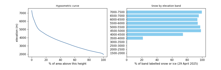
band  share_of_area_%  median_slope_deg  snow_or_ice_%
0   1500-2000              0.5              18.4            0.0
1   2000-2500             22.4              23.3            0.0
2   2500-3000             18.8              35.7            0.1
3   3000-3500             16.0              39.3            0.5
4   3500-4000             14.0              40.8           21.3
5   4000-4500             10.6              40.2           74.5
6   4500-5000              8.0              41.9           98.3
7   5000-5500              3.7              48.7           97.5
8   5500-6000              2.3              52.7           94.1
9   6000-6500              2.2              51.4           93.7
10  6500-7000              1.2              50.2           95.4
11  7000-7500              0.5              44.1           99.5
5.7 A profile across the valley
A profile samples the DEM along a line. Across the Hunza valley it shows the shape carved by ice and water. Rivers cut V-shaped valleys by eroding their beds; glaciers, which fill the valley, widen and deepen it into a U-shape with steep walls and a flatter floor. The Karakoram is one of the fastest-rising mountain ranges on Earth, pushed up by the collision of the Indian and Eurasian plates (about 4 cm per year of convergence across the Himalaya-Karakoram system), and its rivers and glaciers cut down about as fast as it rises, which is why relief here is among the greatest anywhere.
lon = np.linspace(74.60, 74.72, 300)
lat = np.linspace(36.36, 36.27, 300)
cols = ((lon - dtf.c) / dtf.a).astype(int)
rows_ = ((lat - dtf.f) / dtf.e).astype(int)
prof = dem[rows_, cols]
dist = np.concatenate([[0], np.cumsum(np.hypot(np.diff(lon) * 111320 * np.cos(lat0), np.diff(lat) * 110950))]) / 1000
plt.figure(figsize=(7, 2.8))
plt.fill_between(dist, prof, prof.min() - 200, color="#ccbb99")
plt.plot(dist, prof, color="#664422")
plt.xlabel("distance along the line, north-west to south-east (km)")
plt.ylabel("elevation (m)")
plt.title("Profile across the Hunza valley", fontsize=9)
plt.show()
print(f"from {prof.max():,.0f} m to {prof.min():,.0f} m and back over {dist[-1]:.1f} km")
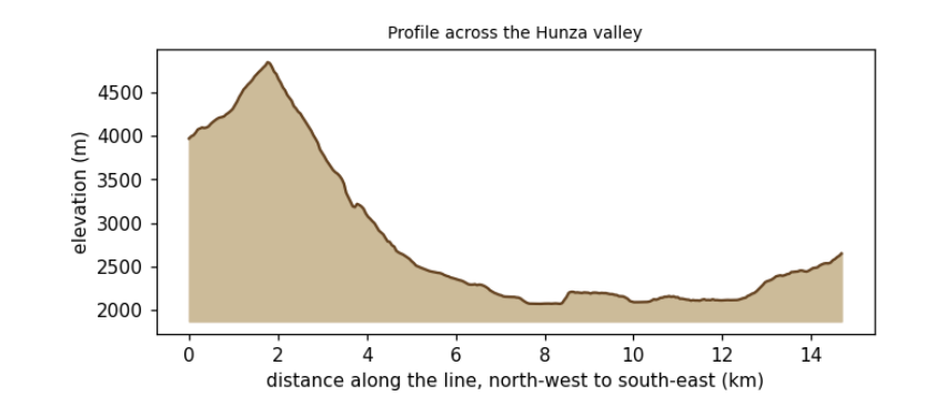
from 4,846 m to 2,073 m and back over 14.7 km
5.8 What to remember
-
A DEM's heights have a datum; know whether it is a surface or a terrain model, and its errors on steep ground.
-
Convert pixel sizes to metres before computing slope; test the formula on a surface with a known answer.
-
Illumination, \(\cos i\), explains much of the brightness in mountain images; correct it before comparing slopes.
-
Report mountain results by elevation band, and remember the lapse rate behind them.
Exercises. (1) Compute slope with numpy's gradient and compare it with Horn's method. (2) Repeat the C-correction for the near-infrared band, using vegetation pixels. (3) Draw a profile along the river instead of across it and estimate its gradient in metres per kilometre.
6. From pixels to answers
6.1 Overview
With clean, aligned images, analysis turns pixels into information: indices that measure a property, maps that sort the ground into classes, numbers that say how good those maps are, and time series that show change. Then post-processing makes the result usable: cleaning speckle, turning pixels into polygons, measuring areas, and drawing a map someone else can read.
What you will learn: spectral indices and the science behind them; classification by thresholds, by clustering (unsupervised) and by a random forest trained on labelled data (supervised); accuracy assessment done properly; sieving, vectorising and measuring areas; a vegetation time series with a trend test; and the parts of a good map.
import importlib.util, subprocess, sys
need = {"pystac_client": "pystac-client", "planetary_computer": "planetary-computer", "rasterio": "rasterio",
        "sklearn": "scikit-learn", "geopandas": "geopandas"}
missing = [p for m, p in need.items() if importlib.util.find_spec(m) is None]
if missing:
    subprocess.run([sys.executable, "-m", "pip", "install", "-q", *missing], check=True)
import os
os.environ.setdefault("LOKY_MAX_CPU_COUNT", "4")
import numpy as np
import pandas as pd
import geopandas as gpd
import matplotlib.pyplot as plt
from matplotlib.colors import ListedColormap
import rasterio
from rasterio.windows import from_bounds
from rasterio.warp import transform_bounds, reproject, Resampling
from rasterio.features import sieve, shapes
from shapely.geometry import shape
from scipy import stats
from sklearn.cluster import KMeans
from sklearn.ensemble import RandomForestClassifier
from sklearn.metrics import confusion_matrix, cohen_kappa_score
import pystac_client, planetary_computer
plt.rcParams.update({"figure.dpi": 110})
catalog = pystac_client.Client.open("https://planetarycomputer.microsoft.com/api/stac/v1", modifier=planetary_computer.sign_inplace)
BBOX = [74.60, 36.29, 74.72, 36.36]                       # Aliabad, Karimabad and the valley floor of central Hunza
6.2 The image and its bands
We use the clearest Sentinel-2 Level-2A image of late summer 2024, when fields and orchards are green and the snow line is high, and stack six bands at 20 m. (The preparation notebook explains each of these steps.)
item = sorted(catalog.search(collections=["sentinel-2-l2a"], bbox=BBOX, datetime="2024-08-01/2024-09-30",
                             query={"eo:cloud_cover": {"lt": 5}}).items(), key=lambda i: i.properties["eo:cloud_cover"])[0]
KEYS = ["B02", "B03", "B04", "B08", "B11", "B12"]
with rasterio.open(item.assets["B11"].href) as s:
    win = from_bounds(*transform_bounds("EPSG:4326", s.crs, *BBOX), s.transform)
    shape20, crs, tf = s.read(1, window=win).shape, s.crs, s.window_transform(win)

def band(key, rule=Resampling.average):
    with rasterio.open(item.assets[key].href) as s:
        w = from_bounds(*transform_bounds("EPSG:4326", s.crs, *BBOX), s.transform)
        return s.read(1, window=w, out_shape=shape20, resampling=rule)

R = {k: (band(k).astype("float32") - 1000) / 10000 for k in KEYS}
scl = band("SCL", Resampling.nearest)
print(item.id[:38], "| cloud", item.properties["eo:cloud_cover"], "% | grid", shape20, "at 20 m, CRS", crs)
S2B_MSIL2A_20240921T054629_R048_T43SDA | cloud 0.780522 % | grid (390, 540) at 20 m, CRS EPSG:32643
6.3 Spectral indices
An index combines bands so that one property stands out and others (overall brightness, illumination) cancel. Most are normalised differences, \((a - b)/(a + b)\), which range from -1 to 1 and are unaffected if both bands are scaled by the same factor, as shadow does.
Index |
Formula (Sentinel-2) |
Why it works |
|---|---|---|
NDVI, vegetation |
(NIR - red) / (NIR + red) |
chlorophyll absorbs red; leaf structure scatters NIR |
NDSI, snow |
(green - SWIR) / (green + SWIR) |
ice is bright in green, absorbs SWIR |
NDWI, open water |
(green - NIR) / (green + NIR) |
water absorbs NIR almost completely |
NBR, burn severity |
(NIR - SWIR2) / (NIR + SWIR2) |
fire removes leaves (NIR falls) and dries soil (SWIR2 rises) |
The chemistry of the red band. Chlorophyll a and b are pigments whose molecules hold a ring of alternating single and double bonds around a magnesium atom. Electrons in such rings are shared across the whole ring, so little energy lifts one to a higher level: exactly the energy of blue (about 430 nm) and red (about 660 nm) photons, which are absorbed and drive photosynthesis. Green light is absorbed less and partly reflected, so leaves look green.
nd = lambda a, b: (R[a] - R[b]) / (R[a] + R[b])
idx = {"NDVI": nd("B08", "B04"), "NDSI": nd("B03", "B11"), "NDWI": nd("B03", "B08")}
fig, ax = plt.subplots(1, 3, figsize=(12, 3.4))
for a, (name, v), cmap in zip(ax, idx.items(), ["YlGn", "Blues", "PuBu"]):
    im = a.imshow(v, cmap=cmap, vmin=-0.5 if name != "NDVI" else 0, vmax=1 if name != "NDVI" else 0.8)
    plt.colorbar(im, ax=a, fraction=0.04)
    a.set_title(name, fontsize=9)
    a.set_axis_off()
plt.tight_layout()
plt.show()
pd.DataFrame({k: pd.Series(v.ravel()).describe(percentiles=[0.05, 0.5, 0.95]) for k, v in idx.items()}).round(3).T
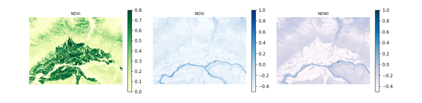
count   mean    std    min     5%    50%    95%    max
NDVI  210600.0  0.258  0.230 -0.870  0.026  0.170  0.752  4.200
NDSI  210600.0 -0.372  0.139 -1.039 -0.557 -0.387 -0.161  0.828
NDWI  210600.0 -0.289  0.197 -2.467 -0.679 -0.229 -0.056  0.938
6.4 Classification 1: thresholds
The simplest map applies rules to indices, in an order that settles overlaps. The thresholds are conventions, not laws (NDSI > 0.4 is the long-standing MODIS snow rule), so a rule-based map should state its rules and be checked like any other. Five classes are enough for this valley.
CLASSES = ["snow and ice", "water", "vegetation", "bare rock and soil", "built-up"]
COLOURS = ["#bbddff", "#2266cc", "#33aa33", "#bb9966", "#dd3333"]
rules = np.full(shape20, 3, "uint8")                                  # default: bare
rules[idx["NDVI"] > 0.35] = 2
rules[(idx["NDWI"] > 0.1) & (idx["NDSI"] < 0.4)] = 1
rules[(idx["NDSI"] > 0.4) & (R["B03"] > 0.2)] = 0
cmap = ListedColormap(COLOURS)
print(pd.Series(np.bincount(rules.ravel(), minlength=5) / rules.size * 100, index=CLASSES).round(1).to_string(), "\n(% of pixels)")
snow and ice           0.1
water                  0.5
vegetation            26.0
bare rock and soil    73.4
built-up               0.0
(% of pixels)
6.5 Classification 2: unsupervised clustering
K-means sorts pixels into k groups so that each pixel is closer (in band space) to its group's centre than to any other. It needs no labels, but it does not know what the groups are: a person must name them afterwards, and one land cover may split across clusters or two may merge. It is useful for exploring an image, not for a final map.
X = np.stack([R[k].ravel() for k in KEYS], axis=1)
km = KMeans(n_clusters=6, n_init=4, random_state=0).fit(X[::7])
clusters = km.predict(X).reshape(shape20)
centres = pd.DataFrame(km.cluster_centers_, columns=KEYS).round(3)
centres["NDVI"] = ((centres.B08 - centres.B04) / (centres.B08 + centres.B04)).round(2)
centres["NDSI"] = ((centres.B03 - centres.B11) / (centres.B03 + centres.B11)).round(2)
centres["share_%"] = (np.bincount(clusters.ravel(), minlength=6) / clusters.size * 100).round(1)
centres
B02    B03    B04    B08    B11    B12  NDVI  NDSI  share_%
0  0.086  0.108  0.119  0.188  0.245  0.223  0.22 -0.39     31.4
1  0.178  0.215  0.238  0.286  0.366  0.357  0.09 -0.26      9.6
2  0.042  0.065  0.055  0.266  0.178  0.121  0.66 -0.47     19.9
3  0.281  0.337  0.371  0.466  0.555  0.532  0.11 -0.24      1.0
4  0.119  0.148  0.168  0.217  0.303  0.291  0.13 -0.34     30.8
5  0.072  0.083  0.084  0.108  0.150  0.137  0.13 -0.29      7.3
6.6 Classification 3: supervised, with reference labels
A supervised classifier learns from pixels whose class is known. Collecting such labels in the field is the gold standard; here we borrow them from ESA WorldCover 2021, a global 10 m land cover map, keeping in mind that it has its own errors (about 75% overall accuracy globally) and a different date, so this shows the method, not a validated map. Its classes are merged into our five.
The classifier is a random forest: many decision trees, each trained on a random sample of pixels and bands, that vote. It handles bands on different scales and non-linear boundaries with little tuning.
Testing honestly. Neighbouring pixels are almost identical, so if training and test pixels are drawn at random from the same image, the test pixels have near-copies in the training set and the accuracy is flattering. The remedy is a spatial split: divide the image into blocks and keep whole blocks for testing.
wc = next(catalog.search(collections=["esa-worldcover"], bbox=BBOX).items())
with rasterio.open(wc.assets["map"].href) as s:
    ref = np.zeros(shape20, "uint8")
    reproject(rasterio.band(s, 1), ref, dst_transform=tf, dst_crs=crs, resampling=Resampling.mode)
WC = {70: 0, 80: 1, 10: 2, 20: 2, 30: 2, 40: 2, 90: 2, 95: 2, 100: 2, 60: 3, 50: 4}   # WorldCover code -> our class
labels = np.vectorize(lambda v: WC.get(int(v), 255))(ref).astype("uint8")
print("WorldCover classes present:", sorted(np.unique(ref).tolist()), "| labelled share", round(np.mean(labels < 255), 3))

block = 40                                                              # 40 x 40 pixels = 800 m blocks
bid = (np.arange(shape20[0])[:, None] // block) * 1000 + (np.arange(shape20[1])[None, :] // block)
rng = np.random.default_rng(0)
test_blocks = rng.choice(np.unique(bid), size=int(0.3 * np.unique(bid).size), replace=False)
is_test = np.isin(bid, test_blocks)
y = labels.ravel()
ok = (y < 255) & np.isfinite(X).all(1)
train = ok & ~is_test.ravel()
test = ok & is_test.ravel()
sample = np.flatnonzero(train)[rng.permutation(train.sum())[:20000]]
rf = RandomForestClassifier(n_estimators=150, min_samples_leaf=3, random_state=0, n_jobs=-1).fit(X[sample], y[sample])
pred = rf.predict(X).reshape(shape20)
print("training pixels", len(sample), "| test pixels", int(test.sum()), "in", len(test_blocks), "held-out blocks")
WorldCover classes present: [10, 30, 40, 50, 60, 70, 80, 100] | labelled share 1.0
training pixels 20000 | test pixels 60800 in 42 held-out blocks
6.7 Accuracy assessment
The confusion matrix counts, for test pixels, the reference class (rows) against the predicted class (columns). From it:
-
overall accuracy: the share on the diagonal;
-
producer's accuracy (recall) for a class: of the pixels that truly are that class, the share mapped correctly (the map-maker's view: what did I miss?);
-
user's accuracy (precision): of the pixels mapped as that class, the share that truly are (the map-user's view: if the map says forest, how often is it?);
-
Cohen's kappa: agreement beyond what chance would give, \(\kappa = (p_o - p_e)/(1 - p_e)\), though many now prefer to report the matrix and per-class accuracies instead.
Rare classes matter: 95% overall accuracy can hide a class mapped entirely wrong. We score the maps on the same held-out blocks, and the random forest also on randomly chosen pixels.
def scores(p, mask):
    cm = confusion_matrix(y[mask], p.ravel()[mask], labels=range(5))
    oa = np.trace(cm) / cm.sum()
    return cm, oa, cohen_kappa_score(y[mask], p.ravel()[mask])

rows = []
for name, m in [("thresholds", rules), ("random forest", pred)]:
    cm, oa, k = scores(m, test)
    rows.append(dict(map=name, test="spatial blocks", overall_accuracy=oa, kappa=k))
rand = ok & (rng.random(ok.size) < 0.3) & ~np.isin(np.arange(ok.size), sample)
cm_r, oa_r, k_r = scores(pred, rand)
rows.append(dict(map="random forest", test="random pixels (flattering)", overall_accuracy=oa_r, kappa=k_r))
print(pd.DataFrame(rows).round(3).to_string(index=False))
cm, oa, k = scores(pred, test)
cmd = pd.DataFrame(cm, index=[f"ref: {c}" for c in CLASSES], columns=[f"map: {c}" for c in CLASSES])
cmd["producer's"] = (np.diag(cm) / cm.sum(1).clip(1)).round(2)
cmd.loc["user's"] = list((np.diag(cm) / cm.sum(0).clip(1)).round(2)) + [round(oa, 2)]
cmd
map                       test  overall_accuracy  kappa
   thresholds             spatial blocks             0.739  0.437
random forest             spatial blocks             0.856  0.714
random forest random pixels (flattering)             0.844  0.705
                         map: snow and ice  map: water  map: vegetation  \
ref: snow and ice                     84.0        7.00             1.00
ref: water                             9.0      511.00            10.00
ref: vegetation                        0.0        0.00         19417.00
ref: bare rock and soil              115.0       94.00          2763.00
ref: built-up                          0.0        0.00           347.00
user's                                 0.4        0.83             0.86

                         map: bare rock and soil  map: built-up  producer's
ref: snow and ice                         347.00            0.0        0.19
ref: water                                189.00            0.0        0.71
ref: vegetation                          4100.00           31.0        0.82
ref: bare rock and soil                 31998.00           27.0        0.91
ref: built-up                             691.00           59.0        0.05
user's                                      0.86            0.5        0.86
Reading the results. The random forest beats the thresholds by a wide margin, partly because the rules have no built-up class at all: every village pixel is wrong by design. Here the random-pixel score is no higher than the spatial one, and the same held when we trained on every pixel of the training blocks (0.852 with a random split against 0.859 with spatial blocks). In this image the ceiling is set by disagreement with the reference map itself, which has its own errors and a different year, not by leakage. Spatial testing matters most when labels come from a few dense patches or the property varies smoothly in space; Ploton et al. (2020, Nature Communications, doi:10.1038/s41467-020-18321-y) showed a published biomass map whose random-split accuracy disappeared under spatial testing. So use spatial splits by default: when leakage is absent they cost nothing, and when present they reveal it.
6.8 Post-processing: sieve, polygons and areas
Pixel classifiers leave speckle: single pixels of one class inside another. A sieve replaces patches smaller than a minimum size with their surroundings; choose the size from the smallest feature you care about (here 6 pixels, about 0.24 ha). Vectorising turns patches into polygons that a GIS can edit and attach attributes to. Areas must be measured in an equal-area or local projected CRS (UTM is fine at this scale), never in degrees.
clean = sieve(pred.astype("uint8"), size=6)
changed = np.mean(clean != pred)
polys = [dict(cls=CLASSES[int(v)], geometry=shape(g)) for g, v in shapes(clean, transform=tf)]
gdf = gpd.GeoDataFrame(polys, crs=crs)
gdf["area_km2"] = gdf.area / 1e6
summary = gdf.groupby("cls").agg(polygons=("area_km2", "size"), area_km2=("area_km2", "sum")).round(2)
print(f"sieve changed {100 * changed:.1f}% of pixels; {len(gdf):,} polygons")
summary
sieve changed 3.8% of pixels; 701 polygons
                    polygons  area_km2
cls
bare rock and soil       366     46.14
snow and ice              15      0.29
vegetation               315     36.69
water                      5      1.12
6.9 A time series and a trend test
Change is found by repeating a measurement over time. We take every Sentinel-2 image of 2018-2025 for a patch of irrigated fields and orchards on the valley floor, mask cloud with the scene classification, and keep the median NDVI of each image. The seasonal cycle (green-up in spring, harvest in autumn, bare in winter) dominates, so to ask whether summers are getting greener or browner we take the July-August median of each year.
Testing for a trend. The Mann-Kendall test asks whether later values tend to be larger (or smaller) than earlier ones, without assuming a straight line or normal errors. For \(n\) values it counts every pair: \(S = \sum_{i<j} \operatorname{sign}(x_j - x_i)\). With no trend, \(S\) has mean 0 and variance \(n(n-1)(2n+5)/18\), so \(Z = (S - \operatorname{sign}S)/\sqrt{\operatorname{Var}S}\) is close to a standard normal, giving a p-value. The Sen slope, the median of the slopes between all pairs, measures the size. A p-value above 0.05 does not mean "no change": it means the record is too short or too variable to tell. With 8 summers, only large trends can be detected.
FIELDS = [74.655, 36.310, 74.675, 36.320]
ts_items = list(catalog.search(collections=["sentinel-2-l2a"], bbox=FIELDS, datetime="2018-01-01/2025-12-31",
                               query={"eo:cloud_cover": {"lt": 40}, "s2:mgrs_tile": {"eq": item.properties["s2:mgrs_tile"]}}).items())
recs = []
for it in ts_items:
    def rd(key, rule=Resampling.average):
        with rasterio.open(it.assets[key].href) as s:
            w = from_bounds(*transform_bounds("EPSG:4326", s.crs, *FIELDS), s.transform)
            return s.read(1, window=w, out_shape=(55, 90), resampling=rule).astype("float32")
    off = -1000 if float(it.properties["s2:processing_baseline"]) >= 4 else 0
    sc = rd("SCL", Resampling.nearest)
    good = np.isin(sc, [4, 5])                                       # vegetation or bare ground: clear land
    if good.mean() < 0.6:
        continue
    nir, red = (rd("B08") + off) / 1e4, (rd("B04") + off) / 1e4
    recs.append(dict(date=pd.Timestamp(it.properties["datetime"][:10]), ndvi=float(np.median(((nir - red) / (nir + red))[good]))))
ts = pd.DataFrame(recs).sort_values("date").reset_index(drop=True)
summer = ts[ts.date.dt.month.isin([7, 8])].groupby(ts.date.dt.year).ndvi.median()
n = len(summer)
s_stat = sum(np.sign(summer.values[j] - summer.values[i]) for i in range(n) for j in range(i + 1, n))
z = (s_stat - np.sign(s_stat)) / np.sqrt(n * (n - 1) * (2 * n + 5) / 18)
p = 2 * stats.norm.sf(abs(z))
sen = np.median([(summer.values[j] - summer.values[i]) / (summer.index[j] - summer.index[i]) for i in range(n) for j in range(i + 1, n)])
print(f"{len(ts_items)} images found, {len(ts)} clear enough; summers: {n}")
print(f"Mann-Kendall S = {s_stat:.0f}, Z = {z:.2f}, p = {p:.3f}; Sen slope {sen * 10:+.3f} NDVI per decade")
print("check against scipy's Kendall tau p:", round(stats.kendalltau(summer.index, summer.values).pvalue, 3))
fig, ax = plt.subplots(1, 2, figsize=(11, 3.2), gridspec_kw={"width_ratios": [2.2, 1]})
ax[0].plot(ts.date, ts.ndvi, ".", ms=4, color="#33aa33")
ax[0].set_ylabel("median NDVI")
ax[0].set_title("Every clear image: the seasonal cycle", fontsize=9)
ax[1].plot(summer.index, summer.values, "o-", color="#226622")
ax[1].set_title(f"July-August median; Sen slope {sen * 10:+.3f}/decade, p = {p:.2f}", fontsize=9)
plt.tight_layout()
plt.show()
258 images found, 240 clear enough; summers: 8
Mann-Kendall S = 4, Z = 0.37, p = 0.711; Sen slope +0.014 NDVI per decade
check against scipy's Kendall tau p: 0.72
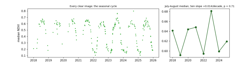
6.10 Making a map someone else can read
A map for others needs: a title saying what and when; a legend naming every colour; a scale bar; a north arrow if north is not up; the source and date of the data; the projection; and colours that people with colour-vision deficiency can tell apart (avoid red against green as the only difference; check with a simulator).
fig, ax = plt.subplots(figsize=(8, 5))
ext = rasterio.transform.array_bounds(*shape20, tf)
ax.imshow(clean, cmap=cmap, vmin=-0.5, vmax=4.5, extent=[ext[0], ext[2], ext[1], ext[3]], interpolation="nearest")
x0, y0 = ext[0] + 600, ext[1] + 500
ax.plot([x0, x0 + 2000], [y0, y0], color="black", lw=3)
ax.text(x0 + 1000, y0 + 200, "2 km", ha="center", fontsize=8)
ax.annotate("N", xy=(ext[2] - 500, ext[3] - 400), xytext=(ext[2] - 500, ext[3] - 1400), ha="center",
            arrowprops=dict(arrowstyle="-|>", color="black"), fontsize=9)
ax.legend([plt.Rectangle((0, 0), 1, 1, color=c) for c in COLOURS], CLASSES, loc="upper left", bbox_to_anchor=(1.01, 1), fontsize=8, frameon=False)
ax.set_title(f"Land cover, central Hunza, {item.properties['datetime'][:10]}", fontsize=10)
ax.set_xlabel(f"Easting (m), {crs}")
ax.set_ylabel("Northing (m)")
ax.text(1.01, 0.02, "Random forest on Sentinel-2 L2A,\ntrained on ESA WorldCover 2021;\nsieved to 6 pixels.", transform=ax.transAxes, fontsize=7)
plt.tight_layout()
plt.show()
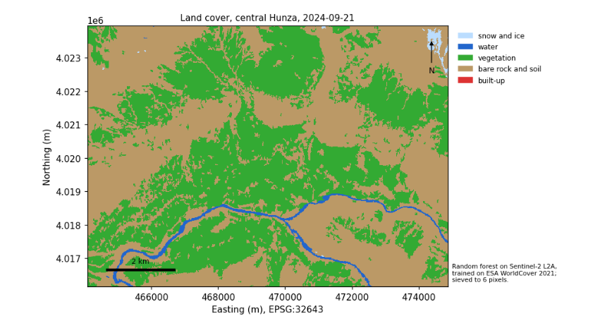
6.11 What to remember
-
Indices work because of physics, chemistry and biology; know which, and their limits.
-
Rules, clusters and trained classifiers each have their place; all must be checked against reference data.
-
Test on spatially separate data, and report the confusion matrix and per-class accuracies, not only one number.
-
Clean speckle, measure areas in a projected CRS, and keep a map's title, legend, scale, source and projection.
-
A trend test says whether a record can show change, not whether change happened: report the slope with the test.
Exercises. (1) Change the block size of the spatial split to 10 and 100 pixels and watch the accuracy. (2) Add NDVI and NDSI as features to the random forest: does accuracy rise? (3) Repeat the time series for a patch of bare hillside and compare its year-to-year variability with the fields.
7. Glossary and next steps
7.1 Glossary
Affine transform
Six numbers that place a raster on a map: pixel size, rotation and the corner’s coordinates.
Atmospheric correction
Removing the effects of scattering and absorption by the air, turning top-of-atmosphere into surface reflectance.
Band
One range of wavelengths recorded by a sensor; one layer of an image.
Black body
An ideal object that absorbs all radiation and emits according to Planck’s law.
COG
Cloud-Optimised GeoTIFF: a GeoTIFF arranged so that programs can read only the part they need over the web.
Composite
An image combining many dates, pixel by pixel, usually by the median of clear observations.
Confusion matrix
A table of reference classes against mapped classes, from which every accuracy measure is computed.
CRS
Coordinate reference system: the ellipsoid, datum and projection that give coordinates their meaning; named by an EPSG code.
DEM, DSM, DTM
Digital elevation, surface and terrain models: heights of whatever is seen first (DSM) or of the bare ground (DTM).
Digital number (DN)
The integer stored in a file, turned into a physical value by a scale factor and offset.
Geoid
The surface the oceans would take under gravity alone; the zero of heights above sea level.
Index
A combination of bands, usually a normalised difference, that isolates one property such as vegetation or snow.
Lapse rate
The fall of air temperature with height: 9.8 K per km for dry rising air, about 6.5 K per km on average.
Mann-Kendall test
A rank-based test for a monotonic trend; the Sen slope gives its size.
Mosaic
Several images joined into one.
NetCDF, HDF
Self-describing file formats for multi-dimensional scientific data.
Reflectance
The fraction of incoming light a surface reflects, from 0 to 1.
Resampling
Assigning values to a new grid: nearest neighbour for categories; bilinear, cubic or average for continuous values.
Resolution
Spatial (pixel size), spectral (bands), temporal (revisit) and radiometric (levels of brightness).
STAC
SpatioTemporal Asset Catalog: the shared standard for describing collections, items and assets of geospatial data.
Topographic correction
Removing the brightness differences caused by slopes facing towards or away from the sun.
UTM
Universal Transverse Mercator: 60 zones, each with its own projection, accurate within the zone.
7.2 Where to go next
-
Satellite images in Python: rasters, vectors, indices, clustering and regridding on a Sentinel-2 image of Belfast.
-
Radar in Python for images that see through cloud, and Climate data in Python for climate records and simple models.
-
Hypothesis testing with climate data for the statistics behind trend tests in depth.
-
The documentation of each service is the final word on its data: NASA Earthdata (
earthdata.nasa.gov), the Copernicus data stores (cds.climate.copernicus.eu), Earth Engine (developers.google.com/earth-engine) and STAC (stacspec.org).