6. Is Karachi sinking? InSAR time series
The radar echo carries a phase as well as a strength. Differencing the phase of two passes measures ground motion to millimetres. Here we build a two-year time series of Karachi’s ground from 68 interferograms, reproduce the core of MintPy in numpy, and find a bowl of subsidence under Korangi and Landhi. Notebook: insar.ipynb. Making a DEM from one InSAR pair is covered in the Karakoram hazard tutorial.
6.1 The question and the data
The first notebook used the strength of the radar echo. This one uses its phase: where in its wave cycle the echo returns. Sentinel-1 passes over the same place every 12 days from almost the same position. If the ground moved a little towards or away from the satellite between two passes, the echo's path changed length and its phase shifted. Differencing the phase of two passes gives an interferogram; a series of interferograms gives a time series of ground motion with millimetre precision.
Karachi pumps groundwater and builds on young coastal sediment, both of which make ground compact and sink. Here we measure it.
Data. 76 interferograms from 31 Sentinel-1 acquisitions (relative orbit 42, ascending, January 2023 to December 2024), processed on demand by the Alaska Satellite Facility's HyP3 service (free with a NASA Earthdata login), at 80 m. The full analysis used MintPy; this notebook works on a 30 × 28 km crop of east Karachi averaged to 160 m, and does the core steps itself in numpy so you can see what MintPy does.
import urllib.request
from pathlib import Path
import numpy as np
import matplotlib.pyplot as plt

plt.rcParams.update({"figure.dpi": 110})
BASE = "https://raw.githubusercontent.com/AhmadAmmar/AhmadAmmar.github.io/main/guides/radar-python/notebooks/data_local/"
F = "karachi_insar_crop.npz"
DATA, LOCAL = Path("data"), Path("data_local")
DATA.mkdir(exist_ok=True)
if not (DATA / F).exists():
    (DATA / F).write_bytes((LOCAL / F).read_bytes() if (LOCAL / F).exists() else urllib.request.urlopen(BASE + F, timeout=300).read())
z = np.load(DATA / F)
unw, coh = z["unw"].astype("float32"), z["coh"].astype("float32")
pairs = [list(p) for p in z["dates"]]          # each row: first date, second date
lam = float(z["wavelength"])
print("interferograms, rows, columns:", unw.shape, " wavelength (m):", round(lam, 4))
ext = [z["x0"] / 1e3, z["x0"] / 1e3 + unw.shape[2] * z["cell"] / 1e3, z["y1"] / 1e3 - unw.shape[1] * z["cell"] / 1e3, z["y1"] / 1e3]
interferograms, rows, columns: (68, 175, 187) wavelength (m): 0.0555
6.2 From phase to millimetres
The radar wave travels to the ground and back, so a change \(\Delta R\) in the one-way distance changes the phase by
With λ = 5.55 cm, one full cycle (2π) is 2.8 cm of motion along the line of sight. The phase is only known modulo 2π (a "wrapped" interferogram shows fringes); HyP3 unwraps it with SNAPHU, adding the right multiple of 2π to make it continuous. Coherence (0 to 1) says how similar the two echoes were: water and moving sand decorrelate (low coherence) and their phase is noise; buildings and bare rock stay coherent.
k = 0
fig, ax = plt.subplots(1, 3, figsize=(15, 4.3))
im = ax[0].imshow(np.angle(np.exp(1j * unw[k])), cmap="twilight", extent=ext); ax[0].set_title(f"wrapped phase {pairs[k][0]}-{pairs[k][1]}")
plt.colorbar(im, ax=ax[0], label="rad")
im = ax[1].imshow(unw[k], cmap="RdBu", extent=ext); ax[1].set_title("unwrapped phase"); plt.colorbar(im, ax=ax[1], label="rad")
im = ax[2].imshow(np.nanmean(coh, 0), cmap="gray", vmin=0, vmax=1, extent=ext); ax[2].set_title("mean coherence")
plt.colorbar(im, ax=ax[2])
for a in ax: a.set_xlabel("easting (km)"); a.set_ylabel("northing (km)")
plt.tight_layout(); plt.show()
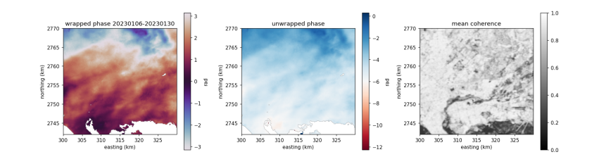
The single interferogram is dominated by smooth patterns tens of kilometres wide: mostly the atmosphere (water vapour delays the wave differently on the two dates) and small orbit errors. Ground motion of a few millimetres in 24 days is hidden underneath. A time series separates them: motion accumulates with time, the atmosphere does not.
6.3 The network of pairs
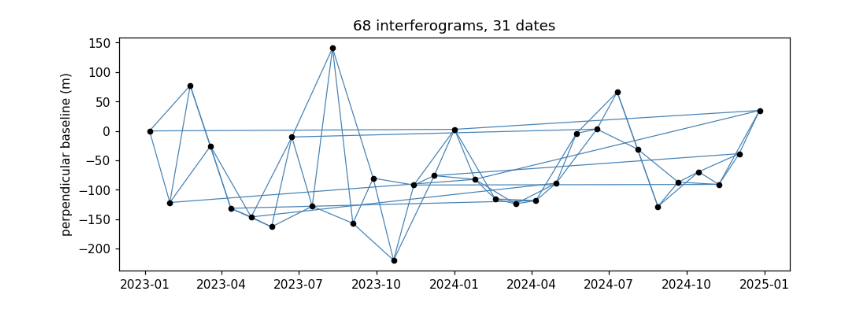
Each interferogram links two dates. Short pairs (24, 48 days) keep coherence high; year-long pairs tie the network across seasons. Pairs with poor average coherence were dropped by MintPy, leaving the network below. The perpendicular baseline is the distance between the two orbits; it controls sensitivity to DEM errors.
import datetime as dt
D = lambda s: dt.datetime.strptime(s, "%Y%m%d")
dates = sorted({d for p in pairs for d in p})
bp = {dates[0]: 0.0}
for (a, b), B in sorted(zip(pairs, z["bperp"]), key=lambda t: t[0][0]):   # approximate per-date baseline for the plot
    bp.setdefault(b, bp.get(a, 0) + float(B))
fig, ax = plt.subplots(figsize=(10, 3.5))
for a, b in pairs:
    ax.plot([D(a), D(b)], [bp.get(a, 0), bp.get(b, 0)], "-", color="steelblue", lw=0.8)
ax.plot([D(d) for d in dates], [bp.get(d, 0) for d in dates], "o", color="k", ms=4)
ax.set_ylabel("perpendicular baseline (m)"); ax.set_title(f"{len(pairs)} interferograms, {len(dates)} dates"); plt.show()
6.4 A reference point
InSAR measures motion relative to somewhere. We pick a reference pixel that is coherent and, according to the full-area MintPy result (referenced to the limestone Mulri hills west of the city), is not moving. Subtracting its phase from every interferogram also removes atmosphere common to the whole crop.
mv = z["mintpy_vel_los_mmyr"]; cm = np.nanmean(coh, 0)
score = np.where((cm > 0.7) & np.isfinite(mv) & np.isfinite(unw).all(0), np.abs(mv), np.inf)   # coherent, unwrapped in every pair, still
r0, c0 = np.unravel_index(np.argmin(score), score.shape)
print(f"reference pixel row {r0}, col {c0}; coherence {cm[r0, c0]:.2f}; MintPy velocity there {mv[r0, c0]:+.2f} mm/yr")
unw_ref = unw - unw[:, r0:r0 + 1, c0:c0 + 1]
reference pixel row 62, col 24; coherence 0.90; MintPy velocity there +0.00 mm/yr
6.5 The small-baseline inversion
Unknowns: the phase at each date relative to the first, \(\phi_1 = 0, \phi_2, \dots, \phi_N\). Each interferogram between dates \(i\) and \(j\) observes \(\phi_j - \phi_i\). Stack these equations into a design matrix \(A\) (one row per interferogram, one column per date after the first, entries −1 and +1) and solve
by least squares, independently for every pixel. With more interferograms than dates the system is redundant, so errors in single interferograms are averaged down. This is the core of the Small BAseline Subset (SBAS) method (Berardino et al., 2002) that MintPy implements.
idx = {d: i for i, d in enumerate(dates)}
A = np.zeros((len(pairs), len(dates) - 1))
for r, (a, b) in enumerate(pairs):
    if idx[a] > 0: A[r, idx[a] - 1] = -1
    if idx[b] > 0: A[r, idx[b] - 1] = 1
print("design matrix", A.shape, " rank", np.linalg.matrix_rank(A), "(must equal the number of unknowns for one connected network)")

n, h, w = unw_ref.shape
Y = unw_ref.reshape(n, -1)
ok = np.all(np.isfinite(Y), axis=0)               # pixels unwrapped in every interferogram
phi = np.full((len(dates) - 1, h * w), np.nan, "float32")
phi[:, ok] = np.linalg.lstsq(A, Y[:, ok], rcond=None)[0]
phi = np.vstack([np.zeros((1, h * w)), phi]).reshape(len(dates), h, w)
disp_mm = -lam / (4 * np.pi) * phi * 1000          # line-of-sight change, mm (negative = away from the satellite)
print("pixels inverted:", ok.sum(), "of", ok.size)
design matrix (68, 30)  rank 30 (must equal the number of unknowns for one connected network)
pixels inverted: 30589 of 32725
6.6 Velocity, and from line of sight to vertical
A straight line through each pixel's time series gives its velocity. Sentinel-1 looks sideways at about 30–45°, so it measures motion along its line of sight (LOS). If the ground only moves vertically, as in compaction-driven subsidence, then vertical = LOS / cos(incidence angle). Motion away from the satellite (negative here) is sinking.
t = np.array([(D(d) - D(dates[0])).days / 365.25 for d in dates])
tt = t - t.mean()
vel_los = np.tensordot(tt, disp_mm - disp_mm.mean(0), axes=(0, 0)) / np.sum(tt ** 2)
vel_up = vel_los / np.cos(np.deg2rad(z["inc_deg"]))
fig, ax = plt.subplots(1, 2, figsize=(13, 4.8))
im = ax[0].imshow(vel_up, cmap="RdBu", vmin=-20, vmax=20, extent=ext); ax[0].set_title("our SBAS: vertical velocity (mm/yr)")
plt.colorbar(im, ax=ax[0])
ax[0].plot(ext[0] + (c0 + .5) * z["cell"] / 1e3, ext[3] - (r0 + .5) * z["cell"] / 1e3, "k^", ms=8, label="reference"); ax[0].legend(loc="lower left")
m = np.isfinite(vel_los) & np.isfinite(mv)
ax[1].hexbin(mv[m] - mv[r0, c0], vel_los[m], gridsize=60, bins="log", extent=(-25, 10, -25, 10))
ax[1].plot([-25, 10], [-25, 10], "r--"); ax[1].set_xlabel("MintPy LOS velocity, re-referenced (mm/yr)"); ax[1].set_ylabel("our LOS velocity (mm/yr)")
ax[1].set_title(f"r = {np.corrcoef(mv[m] - mv[r0, c0], vel_los[m])[0, 1]:.2f}")
plt.tight_layout(); plt.show()
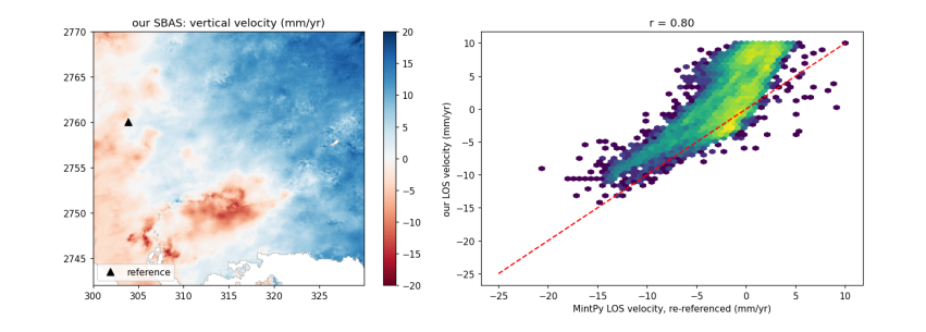
Our ten lines of numpy find the same bowl of subsidence as MintPy (r about 0.8), centred on Korangi and Landhi. But the east of the crop appears to rise steadily, and our velocities sit above MintPy's on the right of the scatter plot. That is a ramp: a tilt across the whole image, left by orbit errors and large-scale atmosphere, that happens to grow over time. Real ground motion is rarely a perfect plane 30 km wide, so the usual remedy is to fit a plane to each date's displacement and remove it. MintPy did this (mintpy.deramp = linear). The cost: a genuine regional tilt would be removed too.
6.7 Removing the ramp
yy, xx = np.mgrid[0:h, 0:w]
G = np.c_[np.ones(h * w), xx.ravel(), yy.ravel()]
good = np.isfinite(disp_mm[-1]).ravel() & (cm.ravel() > 0.7)
disp_dr = disp_mm.copy()
for i in range(len(dates)):
    plane = G @ np.linalg.lstsq(G[good], disp_mm[i].ravel()[good], rcond=None)[0]
    disp_dr[i] = disp_mm[i] - plane.reshape(h, w)
disp_dr -= disp_dr[:, r0:r0 + 1, c0:c0 + 1]          # keep the reference at zero
vel_los2 = np.tensordot(tt, disp_dr - disp_dr.mean(0), axes=(0, 0)) / np.sum(tt ** 2)
vel_up2 = vel_los2 / np.cos(np.deg2rad(z["inc_deg"]))
fig, ax = plt.subplots(1, 2, figsize=(13, 4.8))
im = ax[0].imshow(vel_up2, cmap="RdBu", vmin=-20, vmax=20, extent=ext); ax[0].set_title("deramped: vertical velocity (mm/yr)")
plt.colorbar(im, ax=ax[0])
m = np.isfinite(vel_los2) & np.isfinite(mv)
ax[1].hexbin(mv[m] - mv[r0, c0], vel_los2[m], gridsize=60, bins="log", extent=(-25, 10, -25, 10))
ax[1].plot([-25, 10], [-25, 10], "r--"); ax[1].set_xlabel("MintPy LOS velocity, re-referenced (mm/yr)"); ax[1].set_ylabel("our deramped LOS velocity (mm/yr)")
ax[1].set_title(f"r = {np.corrcoef(mv[m] - mv[r0, c0], vel_los2[m])[0, 1]:.2f}")
plt.tight_layout(); plt.show()
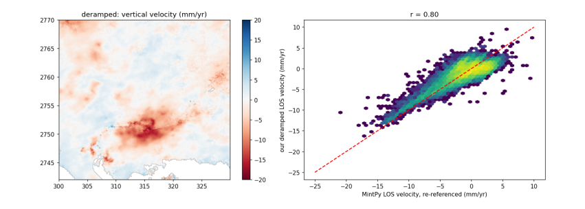
With the ramp gone, the scatter follows the 1:1 line: our values now agree with MintPy in level as well as pattern. The remaining differences come from steps we skipped: MintPy also estimates the DEM error from the baselines, masks pixels whose time series do not fit the network (temporal coherence), and fits the ramp over its whole 55 × 45 km area rather than our crop.
6.8 One pixel through time
r1, c1 = np.unravel_index(np.nanargmin(np.where(cm > 0.7, mv, np.nan)), mv.shape)   # fastest sinking by MintPy
up = disp_dr / np.cos(np.deg2rad(z["inc_deg"]))
fig, ax = plt.subplots(figsize=(9, 3.6))
ax.plot([D(d) for d in dates], up[:, r1, c1], "o-", label=f"fastest-sinking coherent pixel ({vel_up2[r1, c1]:.1f} mm/yr)")
ax.plot([D(d) for d in dates], up[:, r0, c0], "s-", color="grey", label="reference")
ax.set_ylabel("vertical displacement (mm)"); ax.legend(); plt.show()
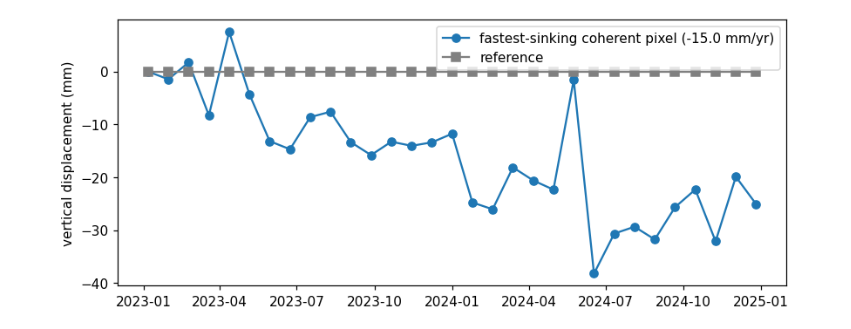
The sinking pixel trends down over the two years, but single dates scatter by a centimetre or more: that scatter is mostly water vapour in the atmosphere on each date, which the network cannot remove because it is different every time. A velocity fitted over two years averages much of it out; more dates, and a tropospheric correction from a weather model such as ERA5, would tighten it further.
6.9 Running the whole thing yourself
The full-area result came from two programs, run from the commons-city repository:
“‘python
6.10 What you have learned
import hyp3_sdk as sdk hyp3 = sdk.HyP3() hyp3.submit_insar_job(reference_granule, secondary_granule, name="karachi", looks="20x4", include_look_vectors=True, include_dem=True, apply_water_mask=True) jobs = hyp3.watch(hyp3.find_jobs(name="karachi")); jobs.download_files("hyp3") “‘
“‘text