The whole guide on one page
1. Before you start
This guide is the notebook version of Reading radar images. That manual explains what radar images show and how they were made in Google Earth Engine; here you work with the images yourself in Python, from opening a file to an area of flooded land with its uncertainty. The images were exported from Earth Engine by the manual’s scripts and are downloaded by the notebook’s first cell, so you need no Earth Engine account.
1.1 What you will learn
-
Data: what a georeferenced raster is (bands, coordinate reference system, pixel size) and how to open one with
rasterio. -
Physics: what a radar measures, why water is dark and buildings bright, what decibels are, what speckle is, and what VV and VH polarisations tell you.
-
Methods: why averages must be taken in linear units, how to measure speckle (the equivalent number of looks), how Otsu’s method chooses a threshold, and how a flood rule is built from two dates and a water record.
-
Reading results: how to read each image, histogram, table and map, and how to report an area with its uncertainty.
1.2 Getting Python and the notebook
Open the Notebooks page of this guide and choose Open in Colab to run it in a web browser with nothing to install; the first cell installs rasterio, which Colab lacks. On your own computer:
conda create -n radar python=3.12 numpy matplotlib rasterio jupyterlab
conda activate radar
jupyter lab
Then open the downloaded radar.ipynb. Boxes labelled In [n] are code and Out [n] what it printed or drew. Run the cells in order from the top.
1.3 Setup
This notebook reads Sentinel-1 radar images with Python. It works the two experiments of the guide Reading radar images step by step: the basics over London, then mapping the 2022 flood in Sindh. The images were exported from Google Earth Engine by the scripts of that guide; here they are small GeoTIFF files, downloaded by the first cell, so no Earth Engine account is needed.
Libraries: rasterio reads and writes georeferenced rasters (GeoTIFF); numpy does arithmetic on whole images; matplotlib draws them. Google Colab does not include rasterio, so the first cell installs it when missing.
import importlib.util, json, subprocess, sys, urllib.request
from pathlib import Path
if importlib.util.find_spec("rasterio") is None:
    subprocess.run([sys.executable, "-m", "pip", "install", "-q", "rasterio"], check=True)
import numpy as np
import rasterio
from rasterio.warp import transform as reproject_points
import matplotlib.pyplot as plt

plt.rcParams.update({"figure.dpi": 110})
BASE = "https://raw.githubusercontent.com/AhmadAmmar/AhmadAmmar.github.io/main/guides/radar-python/notebooks/data_local/"
FILES = ["london_mean_vv_10m.tif", "london_single_vv_10m.tif", "london_2024_mean_80m.tif", "sindh_flood_200m.tif", "london_stats.json", "sindh_stats.json"]
DATA, LOCAL = Path("data"), Path("data_local")
DATA.mkdir(exist_ok=True)
for f in FILES:
    if not (DATA / f).exists():
        (DATA / f).write_bytes((LOCAL / f).read_bytes() if (LOCAL / f).exists() else urllib.request.urlopen(BASE + f, timeout=120).read())
    print(f"{f:28s} {(DATA / f).stat().st_size / 1e6:5.2f} MB")
london_mean_vv_10m.tif        2.85 MB
london_single_vv_10m.tif      2.90 MB
london_2024_mean_80m.tif      4.13 MB
sindh_flood_200m.tif          3.91 MB
london_stats.json             0.00 MB
sindh_stats.json              0.00 MB
2. Radar basics
Before reading any image, it helps to know what a radar measures and why the numbers are in decibels. This chapter then opens the first image and shows why every average must be taken in linear units.
2.1 What a radar image measures
Sentinel-1 is a radar satellite. It sends pulses of microwaves (wavelength about 5.5 cm) sideways and down at the ground and measures how much energy comes back. Because it brings its own illumination, it sees through cloud and at night: that is why it is used for floods, which come with cloud.
What comes back depends on the surface. A smooth surface, such as calm water or a runway, acts like a mirror and sends the pulse away from the satellite: it looks dark. A rough surface, such as a field, scatters energy in all directions, some of it back: medium. Buildings form corners with the ground that send energy straight back: bright. The quantity measured is the backscatter coefficient, σ⁰ (sigma-nought), the share of energy returned per unit area. It spans a huge range, from about 0.001 for calm water to above 10 for a building corner, so it is given in decibels (dB):
Every 10 dB is a factor of ten, every 3 dB roughly a factor of two. Negative dB values are normal: they mean less than the reference, not negative energy.
for lin in [0.001, 0.01, 0.1, 0.5, 1, 2, 10]:
    print(f"linear {lin:7.3f}  ->  {10 * np.log10(lin):+6.1f} dB")
linear   0.001  ->   -30.0 dB
linear   0.010  ->   -20.0 dB
linear   0.100  ->   -10.0 dB
linear   0.500  ->    -3.0 dB
linear   1.000  ->    +0.0 dB
linear   2.000  ->    +3.0 dB
linear  10.000  ->   +10.0 dB
2.2 Open a radar image
A GeoTIFF holds a grid of numbers (one or more bands) and the information that places it on the Earth: the coordinate reference system (CRS) and the transform, which gives the coordinates of the top-left corner and the size of a pixel. Here: the mean VV backscatter (in dB) of all Sentinel-1 scenes of 2024 over central London, at 10 m.
with rasterio.open(DATA / "london_mean_vv_10m.tif") as src:
    vv = src.read(1)
    print("bands:", src.count, "| rows x columns:", src.shape, "| CRS:", src.crs, "| pixel size:", src.res, "m")
    print("left, bottom, right, top:", [round(v) for v in src.bounds])
    london_transform, london_crs = src.transform, src.crs
print(f"values (dB): min {np.nanmin(vv):.1f}, 2nd percentile {np.nanpercentile(vv, 2):.1f}, median {np.nanmedian(vv):.1f}, "
      f"98th percentile {np.nanpercentile(vv, 98):.1f}, max {np.nanmax(vv):.1f}")

def show(img, ax, title, lo=2, hi=98, cmap="gray"):
    """Display with a percentile stretch: the darkest 2% black, the brightest 2% white, the rest in between."""
    a, b = np.nanpercentile(img, [lo, hi])
    ax.imshow(img, cmap=cmap, vmin=a, vmax=b)
    ax.set_title(title, fontsize=9); ax.set_xticks([]); ax.set_yticks([])

fig, ax = plt.subplots(figsize=(7, 5.3))
show(vv, ax, "Mean VV backscatter, 2024, central London (dB)")
plt.tight_layout(); plt.show()
bands: 1 | rows x columns: (806, 1062) | CRS: EPSG:27700 | pixel size: (10.0, 10.0) m
left, bottom, right, top: [524950, 174980, 535570, 183040]
values (dB): min -19.3, 2nd percentile -13.3, median -4.4, 98th percentile 9.8, max 37.2
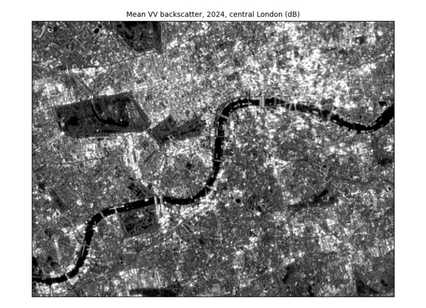
How to read the image. Each pixel is 10 m × 10 m. Grey level is backscatter: dark is low (smooth surfaces), light is high. The values were stretched so the darkest 2% are black and the brightest 2% white; without the stretch a few very bright corners would make the rest look uniformly dark. You can now read London as radar sees it: the Thames is a dark band winding across the middle (smooth water); parks such as Hyde Park are mid-grey (grass and trees); the City and Canary Wharf are the brightest areas (building corners); reservoirs in the west are dark patches.
2.3 Averaging: always in linear units
Because dB is a logarithm, the average of dB values is not the dB of the average. Two pixels at −30 dB (water) and 0 dB (a bright roof): their mean in dB is −15 dB. In linear units they are 0.001 and 1, whose mean is 0.5005, or −3 dB. The dB mean is too dark by 12 dB, a factor of about 16. Every average (over time, over an area, when making pixels bigger) must be taken in linear units and converted back.
pair = np.array([-30.0, 0.0])
print(f"mean of dB values: {pair.mean():.1f} dB;  mean in linear units: {10 * np.log10(np.mean(10 ** (pair / 10))):.1f} dB")
whole_db = np.nanmean(vv)
whole_lin = 10 * np.log10(np.nanmean(10 ** (vv / 10)))
print(f"whole London image: mean of dB values {whole_db:.2f} dB, mean in linear units {whole_lin:.2f} dB, "
      f"difference {whole_lin - whole_db:.2f} dB")
mean of dB values: -15.0 dB;  mean in linear units: -3.0 dB
whole London image: mean of dB values -3.53 dB, mean in linear units 1.72 dB, difference 5.25 dB
Over the whole image the difference is a few dB: the dB mean is biased low because it gives too little weight to the bright pixels. That is large compared with the differences we want to detect, such as a field turning to floodwater.
3. Reading London
London has every kind of surface radar sees: water, parks, an airport and dense towers. Here we measure speckle and use the two polarisations to tell these surfaces apart.
3.1 Speckle: why one image is noisy
Each radar pixel adds up echoes from many small scatterers within it. They interfere, sometimes adding and sometimes cancelling, so even a uniform field shows a grainy pattern called speckle. It is not noise in the instrument; it is part of how coherent radar works. Averaging many images (or many neighbouring pixels) reduces it. The equivalent number of looks (ENL) measures how smooth a uniform area is: ENL = mean² / variance of the linear values. One raw Sentinel-1 image has an ENL of about 4–5; averaging n independent images multiplies it by about n.
with rasterio.open(DATA / "london_single_vv_10m.tif") as src:
    one = src.read(1)
stats_l = json.loads((DATA / "london_stats.json").read_text())
def block_enl(img_db, k=8):
    """ENL = mean² / variance of linear values, in every k x k block of pixels."""
    lin = 10 ** (img_db / 10)
    h, w = lin.shape[0] // k * k, lin.shape[1] // k * k
    b = lin[:h, :w].reshape(h // k, k, w // k, k).transpose(0, 2, 1, 3).reshape(-1, k * k)
    b = b[np.isfinite(b).all(axis=1)]
    return b.mean(axis=1) ** 2 / b.var(axis=1)

#### ENL only means something in uniform areas, so use the most uniform blocks: the top 10% of block ENL values
e_one, e_mean = np.percentile(block_enl(one), 90), np.percentile(block_enl(vv), 90)
print(f"ENL in the most uniform 80 m blocks: one scene {e_one:.1f}, mean of {stats_l['nScenesLondon']} scenes {e_mean:.1f} "
      f"({e_mean / e_one:.1f} times smoother)")
print(f"(the manual, over a uniform area: ENL {stats_l['enlOne']} for one scene, {stats_l['enlMany']} for the mean)")
lon, lat = -0.165, 51.507                                   # Hyde Park, for the zoom below
x, y = reproject_points("EPSG:4326", london_crs, [lon], [lat])
row, col = rasterio.transform.rowcol(london_transform, x[0], y[0])

fig, axes = plt.subplots(1, 2, figsize=(8, 3.6))
zoom = (slice(row - 100, row + 100), slice(col - 150, col + 150))
show(one[zoom], axes[0], f"One scene, {stats_l['sceneDate']}")
show(vv[zoom], axes[1], f"Mean of {stats_l['nScenesLondon']} scenes, 2024")
plt.tight_layout(); plt.show()
ENL in the most uniform 80 m blocks: one scene 4.5, mean of 149 scenes 8.8 (1.9 times smoother)
(the manual, over a uniform area: ENL 4.4 for one scene, 20.9 for the mean)
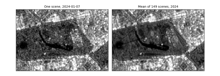
How to read the figure. Both panels show the same 2 km × 3 km around Hyde Park with the same stretch. On the left, one image: grainy, so single pixels cannot be trusted. On the right, the mean of a year: the speckle has averaged out and paths, the lake and building edges are clear. The printed ENL says the same in numbers: in the most uniform blocks, the year's mean is about twice as smooth as one scene. That is far less than 149 scenes might suggest, for two reasons: central London has few truly uniform areas, so even the "most uniform" blocks contain real variation; and scenes taken from the same orbit are not independent views. Over a uniform field the manual measured a much larger gain. What it means in practice: compare averages of several images, or average neighbouring pixels, before drawing conclusions from single pixels; that costs time resolution or spatial detail.
3.2 Polarisation: VV, VH and their difference
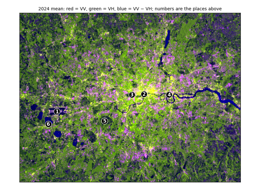
Sentinel-1 sends vertically polarised pulses and records two returns. VV (vertical in, vertical out) is strong from surfaces and corners. VH (vertical in, horizontal out) needs the wave's polarisation to be twisted, which happens mostly through repeated scattering inside volumes such as tree canopies and crops. So VV − VH (in dB) is small for vegetation (a lot of twisted return) and large for smooth surfaces and buildings.
with rasterio.open(DATA / "london_2024_mean_80m.tif") as src:
    vv80, vh80, ratio80 = src.read()
    t80 = src.transform
places = [("Heathrow Airport", -0.46, 51.47), ("River Thames, central London", -0.118, 51.508), ("Hyde Park", -0.165, 51.507),
          ("Canary Wharf", -0.02, 51.505), ("Richmond Park", -0.275, 51.445), ("Reservoir south-west of Heathrow", -0.495, 51.44)]
xs, ys = reproject_points("EPSG:4326", london_crs, [p[1] for p in places], [p[2] for p in places])
def place_mean(img_db, r, c, k=1):
    """Mean of a (2k+1) x (2k+1) window around a pixel, in linear units, back in dB: one pixel can land on a pond or a path."""
    w = img_db[r - k:r + k + 1, c - k:c + k + 1]
    return 10 * np.log10(np.nanmean(10 ** (w / 10)))
rows_ = []
for (name, _, _), xx, yy in zip(places, xs, ys):
    r, c = rasterio.transform.rowcol(t80, xx, yy)
    v, h = place_mean(vv80, r, c), place_mean(vh80, r, c)
    rows_.append((name, v, h, v - h))
print(f"{'place (240 m window)':34s} {'VV dB':>7s} {'VH dB':>7s} {'VV-VH':>6s}")
for name, v, h, d in rows_:
    print(f"{name:34s} {v:7.1f} {h:7.1f} {d:6.1f}")
print("\nbrightest VV:", max(rows_, key=lambda r: r[1])[0], "| darkest VV:", min(rows_, key=lambda r: r[1])[0],
      "| smallest VV-VH (most vegetation-like):", min(rows_, key=lambda r: r[3])[0])

def scale(a):
    lo, hi = np.nanpercentile(a, [2, 98]); return np.clip((a - lo) / (hi - lo), 0, 1)
rgb = np.dstack([scale(vv80), scale(vh80), scale(ratio80)])
fig, ax = plt.subplots(figsize=(7, 5.3))
ax.imshow(rgb); ax.set_xticks([]); ax.set_yticks([])
for k, ((name, _, _), xx, yy) in enumerate(zip(places, xs, ys), 1):
    r, c = rasterio.transform.rowcol(t80, xx, yy)
    ax.annotate(str(k), (c, r), color="white", fontsize=10, ha="center", va="center", fontweight="bold",
                bbox=dict(boxstyle="circle,pad=0.15", fc="black", ec="white", lw=0.8))
ax.set_title("2024 mean: red = VV, green = VH, blue = VV − VH; numbers are the places above", fontsize=9)
plt.tight_layout(); plt.show()
place (240 m window)                 VV dB   VH dB  VV-VH
Heathrow Airport                       9.5    -1.4   10.9
River Thames, central London          -9.2   -15.8    6.6
Hyde Park                             -6.9   -14.0    7.1
Canary Wharf                          13.9     4.6    9.3
Richmond Park                        -12.1   -18.1    6.0
Reservoir south-west of Heathrow     -12.8   -22.0    9.3

brightest VV: Canary Wharf | darkest VV: Reservoir south-west of Heathrow | smallest VV-VH (most vegetation-like): Richmond Park
How to read the table. Each row is one place; the columns are the mean VV and VH backscatter in dB and their difference, each averaged over a 240 m window (in linear units) because a single pixel can fall on a pond or a path. Compare rows rather than reading single numbers: the line under the table names the brightest and darkest place and the one with the smallest VV − VH. Expect open water to be darkest, dense buildings and the airport's hard surfaces and hangars brightest, and vegetated parks to have the smallest difference, because their canopies twist the polarisation. Where a place does not fit (a park reading as dark as water), look at the image: its window may include a lake.
How to read the false-colour image. Each colour channel shows one band, stretched from its darkest 2% to its brightest 2%: red is VV, green is VH, blue is VV − VH. Colours mix as on a screen, so read them by asking which bands are high. Dark blue (the Thames, the reservoirs): VV and VH both very low but their difference large, the signature of smooth water. Green (parks, fields, woods): relatively strong VH, the twisted return from vegetation. Yellow to white (central London, Canary Wharf): VV and VH both high, from building corners and clutter. Purple to pink: high VV with a large difference, typical of smooth hard surfaces and buildings facing the satellite, such as runways and warehouses. The numbered circles are the six places in the table.
4. Mapping a flood: Sindh, 2022
4.1 Two dates, one question
In August and September 2022 extreme monsoon rain flooded a third of Pakistan. Cloud hid the ground from optical satellites for weeks; radar kept seeing. Floodwater is smooth, so it turns dark. The method: take the mean VV of the same weeks in a normal year (2021) and in the flood year (2022), find a threshold that separates dark water from land, and call a pixel flooded if it is darker than the threshold in 2022, was not in 2021, and is not normally water.
with rasterio.open(DATA / "sindh_flood_200m.tif") as src:
    pre, post, occurrence = src.read()
    pixel_km2 = abs(src.res[0] * src.res[1]) / 1e6
print(f"grid {pre.shape}, pixel {src.res[0]:.0f} m = {pixel_km2:.2f} km²; mapped area {np.isfinite(post).sum() * pixel_km2:,.0f} km²")

fig, axes = plt.subplots(1, 2, figsize=(9, 4))
show(pre, axes[0], "Mean VV, 25 Aug–15 Sep 2021 (dB)")
show(post, axes[1], "Mean VV, 25 Aug–15 Sep 2022 (dB)")
plt.tight_layout(); plt.show()
grid (781, 653), pixel 200 m = 0.04 km²; mapped area 20,400 km²
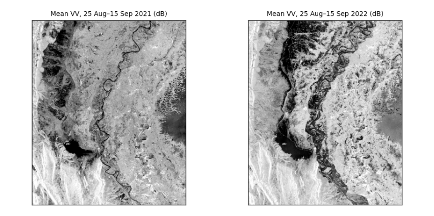
How to read the two images. Same area, same weeks of the year, same stretch. Dark is smooth: in 2021 the dark areas are the Indus and Manchar Lake; in 2022 large new dark areas spread across the plains west of the river. The difference between the panels is the flood.
4.2 Choosing the threshold from the data
In the 2022 image the pixels form two groups, water (dark) and land (brighter). Otsu's method tries every possible threshold t and keeps the one that makes the two groups most distinct, by maximising the between-group variance:
where w₀ and w₁ are the shares of pixels below and above t, and μ₀ and μ₁ their means.
def otsu(values, bins=256):
    v = values[np.isfinite(values)]
    count, edges = np.histogram(v, bins=bins)
    mids = (edges[:-1] + edges[1:]) / 2
    w0 = np.cumsum(count) / count.sum()                  # share below each candidate threshold
    m0 = np.cumsum(count * mids) / count.sum()           # running sum of the means
    mean_all = m0[-1]
    between = (mean_all * w0 - m0) ** 2 / (w0 * (1 - w0) + 1e-12)
    return float(mids[np.argmax(between)])

t = otsu(post)
stats_s = json.loads((DATA / "sindh_stats.json").read_text())
print(f"Otsu threshold on this 200 m grid: {t:.1f} dB (the manual, on the 100 m grid: {stats_s['threshold']} dB)")
fig, ax = plt.subplots(figsize=(7, 2.8))
ax.hist(post[np.isfinite(post)], bins=150, color="#64748b")
ax.axvline(t, color="#b91c1c", lw=1.5, label=f"Otsu threshold {t:.1f} dB")
ax.set(xlabel="VV backscatter, 2022 (dB)", ylabel="pixels", title="Two groups: water on the left, land on the right")
ax.legend(frameon=False, fontsize=8); plt.tight_layout(); plt.show()
Otsu threshold on this 200 m grid: -13.8 dB (the manual, on the 100 m grid: -14.1 dB)
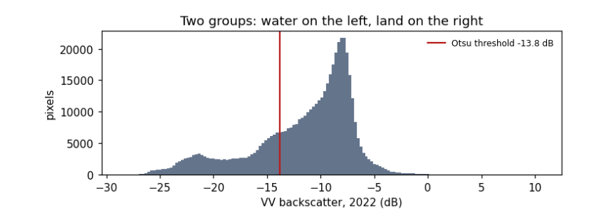
How to read the histogram. x: backscatter in dB; y: how many pixels have that value. Two humps: a smaller one on the left (dark, smooth: water) and a larger one on the right (land). The red line is the threshold Otsu's method chose, in the valley between them. It differs slightly from the manual's because coarser pixels mix water and land at the edges and shift the humps; that difference is a first hint of how uncertain the flood area is.
4.3 From threshold to flood map and area
A pixel is flooded if it is below the threshold in 2022, was above it in 2021, and is water less than 50% of the time in the JRC Global Surface Water record (so permanent rivers and lakes are excluded).
water22, water21 = post < t, pre < t
permanent = occurrence >= 50
flood = water22 & ~water21 & ~permanent
area = flood.sum() * pixel_km2
print(f"flooded: {area:,.0f} km²  (the manual on 100 m pixels: {stats_s['floodKm']:,} km²; the difference comes from the coarser pixels)")
print(f"water already there in 2021: {(water21 & water22).sum() * pixel_km2:,.0f} km²; permanent water: {permanent.sum() * pixel_km2:,.0f} km²")
for dt in (-1.0, +1.0):
    alt = (post < t + dt) & ~(pre < t + dt) & ~permanent
    print(f"threshold {t + dt:.1f} dB -> {alt.sum() * pixel_km2:,.0f} km²  ({100 * (alt.sum() * pixel_km2 / area - 1):+.0f}%)")

fig, ax = plt.subplots(figsize=(7, 5.6))
show(post, ax, "Sindh, September 2022: flood (red) and usual water (blue) over 2022 VV")
over = np.zeros((*post.shape, 4))
over[flood] = [0.85, 0.1, 0.1, 0.75]; over[water21 & water22] = [0.1, 0.35, 0.9, 0.75]
ax.imshow(over); plt.tight_layout(); plt.show()
flooded: 3,283 km²  (the manual on 100 m pixels: 3,458 km²; the difference comes from the coarser pixels)
water already there in 2021: 2,102 km²; permanent water: 324 km²
threshold -14.8 dB -> 3,148 km²  (-4%)
threshold -12.8 dB -> 3,278 km²  (-0%)
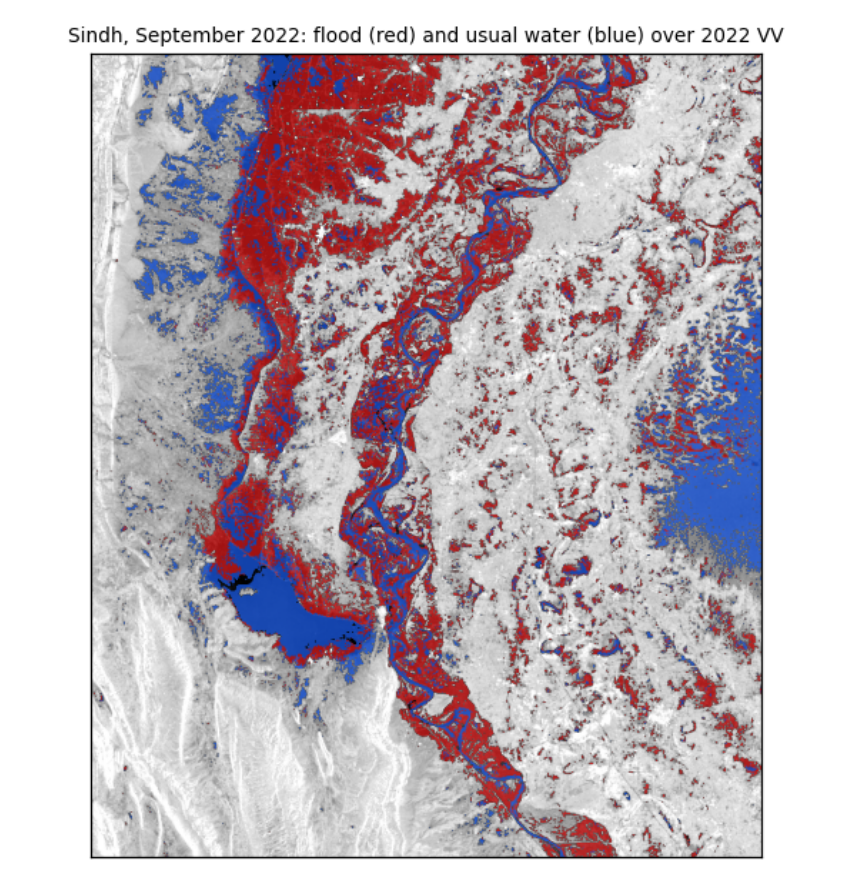
How to read the map. The grey background is the 2022 radar image. Red pixels met all three flood rules: new water in 2022. Blue pixels were water in both years. The red areas spread west of the Indus around Manchar Lake and across the plains of Dadu district, which matches reported flooding there.
What the numbers say. The flooded area is a few thousand km², close to the manual's estimate on finer pixels. Moving the threshold by 1 dB changes the area by only a few percent, and not symmetrically. That is because the rule uses the same threshold for both years: raising it adds water in 2022, but also in 2021, which is then excluded, so the two changes partly cancel. Report the area with this range; it is the honest uncertainty of a threshold method, and it leaves out the larger errors listed next.
What they do not say. Radar misses water under trees and between buildings (the beam does not reach it), can mistake smooth sand or tarmac for water, and sees only the dates it passed over. Pixels are not independent, so area counts are not "samples" for statistical tests (see the guide Hypothesis testing with climate data).
4.4 What you have learned
You opened georeferenced radar images and read their size, grid and coordinates; converted between dB and linear units and saw why averaging must be done in linear units; measured speckle and how averaging reduces it; used two polarisations to tell water, vegetation and buildings apart; chose a threshold from the data with Otsu's method; and mapped a flood with an area and its uncertainty.