7. Testing the tests
The third notebook, climate_data_robustness.ipynb, removes the shortcuts of the second. It reads the daily archive the original study used and compares it with the monthly one, station by station; it builds a homogenisation method from scratch (the Standard Normal Homogeneity Test, tested first on made-up data) and compares the result with NOAA’s and with Berkeley Earth’s; it runs the energy-balance model with 135 combinations of sensitivity and timescales; it reads ten runs each of two climate models to measure chance; and it computes the trend for every start year and window length. Run the second notebook first, or let this one download what it needs.
7.1 The plan
The second notebook ended with its own list of shortcuts: it used monthly station data although the original study used daily maximum and minimum temperatures; it trusted NOAA's corrections instead of making our own; its simple climate model had fixed timescales; it used one run per climate model; and everything used the study's 42-year windows. This notebook removes each shortcut in turn:
-
Daily data. Read the daily archive itself and build monthly and annual means from it.
-
Our own homogenisation. Write a break-detection method from scratch, test it on made-up data, then apply it to the real stations and compare with NOAA's and with an independent group's (Berkeley Earth).
-
Model timescales. Run the energy-balance model 135 times with different settings.
-
Many runs per model. Separate chance from model differences.
-
Window choice. Compute the trend for every possible start year and window length.
It reuses the data folder of the second notebook (run that one first, or let this one download what it needs). The full analysis behind the essay used all 1,155 of the study's stations (2.5 GB of daily files); here we use 40 of them so the notebook runs in minutes.
import io
import tarfile
import time
import urllib.request
from pathlib import Path

import numpy as np
import pandas as pd
import matplotlib.pyplot as plt

pd.set_option("display.width", 110)
plt.rcParams.update({"figure.dpi": 110, "axes.spines.top": False, "axes.spines.right": False})
DATA = Path("data")
(DATA / "daily").mkdir(parents=True, exist_ok=True)
WINDOWS = [(1857, 1898), (1899, 1940), (1941, 1982), (1983, 2024)]
rng = np.random.default_rng(7)
t_start = time.time()


def get(name, url):
    target = DATA / name
    if not target.exists():
        req = urllib.request.Request(url, headers={"User-Agent": "climate-data-notebook/1.0"})
        target.write_bytes(urllib.request.urlopen(req, timeout=600).read())
    return target


def trend(years, values):
    years, values = np.asarray(years, float), np.asarray(values, float)
    ok = ~np.isnan(values)
    x, y = years[ok] - years[ok].mean(), values[ok]
    return 10 * (x * y).sum() / (x * x).sum()


def window_trends(s):
    return {f"{a}-{b}": trend(s.loc[a:b].index, s.loc[a:b].values) for a, b in WINDOWS}


print("ready")
ready
trend here returns only the slope in °C per decade; the second notebook shows how to attach an uncertainty.
7.2 Daily data
What a daily record looks like
GHCN-Daily keeps one text file per station, <station id>.dly. Each line holds one month of one element: TMAX (the day's highest temperature), TMIN (lowest), PRCP (precipitation) and many others. After the 21-character header come 31 blocks of 8 characters, one per day: a 5-character value in tenths of a degree (so 253 is 25.3 °C), then three flags. The second flag is again the quality-control flag; -9999 means missing.
We pick 40 of the study's stations, 20 in the US and 20 elsewhere, at random but reproducibly (the random generator has a fixed seed, 7, so everyone gets the same 40).
inv = pd.read_fwf(get("ghcnd-inventory.txt", "https://www.ncei.noaa.gov/pub/data/ghcn/daily/ghcnd-inventory.txt"),
                  widths=[11, 9, 10, 5, 5, 5], names=["id", "lat", "lon", "element", "first", "last"])
tt = inv[inv.element.isin(["TMAX", "TMIN"])]
per = tt.groupby("id").agg(n=("element", "nunique"), first=("first", "max"), last=("last", "min"), lat=("lat", "first"), lon=("lon", "first"))
sample = per[(per.n == 2) & (per["first"] <= 1900) & (per["last"] >= 2020)]
us_ids = sample.index[sample.index.str.startswith("US")]
other = sample.index[~sample.index.str.startswith("US")]
pick = sorted(rng.choice(us_ids, 20, replace=False).tolist() + rng.choice(other, 20, replace=False).tolist())
for sid in pick:
    get(f"daily/{sid}.dly", f"https://www.ncei.noaa.gov/pub/data/ghcn/daily/all/{sid}.dly")
print(len(sample), "stations in the study's selection; downloaded", len(pick))
print(open(DATA / f"daily/{pick[0]}.dly").readline()[:70])
1155 stations in the study's selection; downloaded 40
ASN00023000183901PRCP    0  a    0  a    0  a   20  a    0  a    0  a
From days to months to years
The rules matter, so they are written out:
-
a day counts only if it has both
TMAXandTMIN, neither is flagged, and the maximum is not below the minimum; -
the day's mean temperature is (TMAX + TMIN) / 2, the convention in most national records;
-
a month counts if it has at least 25 such days (a month with only ten days of data could miss a cold spell);
-
a year counts if all 12 months count.
def daily_to_annual(sid):
    rec = {}
    for line in open(DATA / f"daily/{sid}.dly"):
        el = line[17:21]
        if el not in ("TMAX", "TMIN"):
            continue
        v = np.array([int(line[21 + 8 * d: 26 + 8 * d]) for d in range(31)], float)
        flagged = np.array([line[27 + 8 * d] != " " for d in range(31)])
        v[(v == -9999) | flagged] = np.nan
        rec[(int(line[11:15]), int(line[15:17]), el)] = v / 10
    months = []
    for (y, m, el), tmax in rec.items():
        if el == "TMAX" and (y, m, "TMIN") in rec:
            tmin = rec[(y, m, "TMIN")]
            ok = ~np.isnan(tmax) & ~np.isnan(tmin) & (tmax >= tmin)
            if ok.sum() >= 25:
                months.append((y, m, tmax[ok].mean(), tmin[ok].mean()))
    mo = pd.DataFrame(months, columns=["year", "month", "tmax", "tmin"])
    yr = mo.groupby("year").agg(n=("month", "size"), tmax=("tmax", "mean"), tmin=("tmin", "mean"))
    yr = yr[yr.n == 12].drop(columns="n")
    yr["t"] = (yr.tmax + yr.tmin) / 2
    return yr.assign(id=sid).reset_index()


daily = pd.concat([daily_to_annual(s) for s in pick])
print(daily.groupby("id").year.agg(["min", "max", "size"]).head())
min   max  size
id
ASN00023000  1888  2025    98
ASN00026026  1886  2024   117
AU000011801  1877  2025   136
BKM00014652  1898  2005    60
CAN01018610  1899  2003    99
Daily against monthly, station by station
The monthly archive of notebook 2 is built from the same observations. For each station and the years both have, compare the 1983-2024 trend from our daily calculation with the one from the monthly file.
def open_member(kind, ending):
    tar = tarfile.open(get(f"ghcnm_{kind}.tar.gz", f"https://www.ncei.noaa.gov/pub/data/ghcn/v4/ghcnm.tavg.latest.{kind}.tar.gz"))
    member = next(m for m in tar.getmembers() if m.name.endswith(ending))
    return io.TextIOWrapper(tar.extractfile(member), encoding="ascii")


def monthly_annual(kind):
    cache = DATA / f"ghcnm_{kind}_annual.csv"
    if not cache.exists():
        rows = []
        for line in open_member(kind, ".dat"):
            v = [int(line[19 + 8 * m: 24 + 8 * m]) for m in range(12)]
            if -9999 in v or any(line[25 + 8 * m] != " " for m in range(12)):
                continue
            rows.append((line[:11], int(line[11:15]), sum(v) / 1200))
        pd.DataFrame(rows, columns=["id", "year", "t"]).to_csv(cache, index=False)
    return pd.read_csv(cache)


raw, noaa = monthly_annual("qcu"), monthly_annual("qcf")
both = daily.merge(raw, on=["id", "year"], suffixes=("_daily", "_monthly"))
both = both[both.year.between(1983, 2024)]
cmp_ = both.groupby("id").filter(lambda g: len(g) >= 30).groupby("id").apply(
    lambda g: pd.Series({"daily": trend(g.year, g.t_daily), "monthly": trend(g.year, g.t_monthly)}), include_groups=False)
print(cmp_.round(3).head(8))
print("\nmedian 1983-2024 trend (°C/decade):", cmp_.median().round(3).to_dict())

fig, ax = plt.subplots(figsize=(4.4, 4.2))
ax.scatter(cmp_.monthly, cmp_.daily, s=14, c=np.where(cmp_.index.str.startswith("US"), "#b91c1c", "#1f5c7a"))
lim = [cmp_.min().min() - 0.05, cmp_.max().max() + 0.05]
ax.plot(lim, lim, color="0.6", lw=0.8)
ax.set(xlabel="trend from monthly file", ylabel="trend from daily file", title="1983-2024, one dot per station")
plt.tight_layout()
plt.show()
daily  monthly
id
ASN00026026  0.010    0.010
AU000011801  0.532    0.223
HRE00105203  0.553    0.552
RSM00025551  0.542    0.538
RSM00034110  0.574    0.564
SIM00014015  0.662    0.662
SW000010537  0.582    0.584
SWE00139148  0.533    0.535

median 1983-2024 trend (°C/decade): {'daily': 0.357, 'monthly': 0.321}
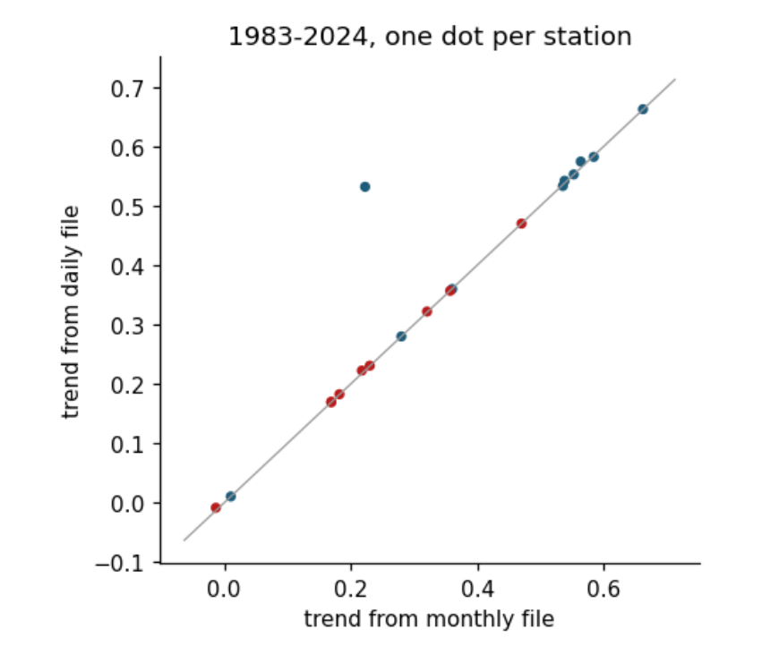
Reading it: each dot is one station (red: US); the grey line is where the two would be equal. Most dots sit on the line: for the same station and the same years, daily and monthly data usually give the same trend. The few that do not are worth a closer look: the monthly archive merges several source collections, so for some stations its record is not built only from the daily file. Across all 1,155 of the study's stations the medians agree to within 0.02 °C per decade, so using monthly data was not a shortcut that changed the answer.
One trap in the daily archive
There is one difference, and it is worth knowing about. Count how many non-US stations have a complete year in each archive.
nonus = lambda d: d[~d.id.str.startswith("US")].groupby("year").id.nunique()
counts = pd.DataFrame({"daily": nonus(daily), "monthly": nonus(raw[raw.id.isin(pick)])}).loc[[1960, 1990, 2010, 2015, 2020, 2024]]
print(counts)
daily  monthly
year
1960   17.0       12
1990   16.0       14
2010   14.0       14
2015   14.0       12
2020   13.0       13
2024    9.0       12
Recent years of many non-US stations in the daily archive have gaps (a few missing days in some month), so they fail the complete-year rule and drop out; the monthly archive fills the same months from other sources. Because stations outside the US warmed faster recently, an average over the daily archive that loses them is pulled down for the last decade. In the full set of the study's stations this lowers the area-weighted 1983-2024 trend from 0.30 (monthly) to 0.24 °C per decade (daily). The lesson: check which stations enter an average in each year, not only how many.
7.3 Our own homogenisation
The idea
A station's record mixes three things: the regional climate, local weather noise, and artificial steps when something about the measurement changed. Neighbouring stations share the regional climate and most of the weather. So subtract a reference series, the average of well-correlated neighbours, from the station: the climate cancels, and what is left is noise plus the station's own steps. A step then shows as a sudden, lasting change in the level of this difference series.
The Standard Normal Homogeneity Test (SNHT)
Alexandersson's test (1986) asks: if we split the difference series at year k, how different are the means before and after? With the series standardised to mean 0 and standard deviation 1 (values \(z_i\)), and \(\bar z_1\), \(\bar z_2\) the means of the first k and the last n − k values,
\(T(k)\) is large where the split separates two different levels. The largest \(T\) marks the most likely break. To decide whether it is real, compare it with what pure noise gives: we simulate 1,000 series of random numbers of the same length and take the value exceeded by only 5 % of them (the critical value). To find several breaks, we split the series at the first break and test each part again (binary segmentation).
def snht(z):
    n = len(z)
    z = (z - z.mean()) / z.std()
    cs = np.cumsum(z)
    k = np.arange(1, n)
    T = k * (cs[:-1] / k) ** 2 + (n - k) * ((cs[-1] - cs[:-1]) / (n - k)) ** 2
    T[:4] = 0; T[-5:] = 0                     # each side needs at least 5 years
    return T.max(), int(T.argmax()) + 1


_crit = {}
def critical(n):
    if n not in _crit:
        _crit[n] = np.percentile([snht(rng.normal(size=n))[0] for _ in range(1000)], 95)
    return _crit[n]


def find_breaks(d):
    found, todo = [], [(0, len(d))]
    while todo:
        a, b = todo.pop()
        if b - a < 10:
            continue
        T, k = snht(d[a:b])
        if T > critical(b - a):
            found.append(a + k)
            todo += [(a, a + k), (a + k, b)]
    return sorted(found)


## test on made-up data: noise, plus a 0.5 °C drop after year 60 and a 0.3 °C rise after year 100
fake = rng.normal(0, 0.25, 140)
fake[60:] -= 0.5
fake[100:] += 0.3
print("breaks found at", find_breaks(fake), "(true: 60 and 100)")
print("critical value for n = 140:", round(critical(140), 2))
breaks found at [60, 96] (true: 60 and 100)
critical value for n = 140: 9.34
On data where we know the answer, the method finds both steps we put in, the second a few years from its true position (noise makes the exact year uncertain). That is the first check any method should pass.
fig, axs = plt.subplots(2, 1, figsize=(8, 4.4), sharex=True)
axs[0].plot(fake, color="0.4", lw=0.8)
for b in find_breaks(fake):
    axs[0].axvline(b, color="#b91c1c", lw=1)
axs[0].set_ylabel("made-up difference (°C)")
z = (fake - fake.mean()) / fake.std(); cs = np.cumsum(z); k = np.arange(1, len(z))
axs[1].plot(k, k * (cs[:-1] / k) ** 2 + (len(z) - k) * ((cs[-1] - cs[:-1]) / (len(z) - k)) ** 2, color="#1f5c7a")
axs[1].axhline(critical(len(z)), color="0.5", ls=":", label="95 % critical value")
axs[1].set(xlabel="year", ylabel="T(k)")
axs[1].legend(frameon=False, fontsize=8)
plt.tight_layout()
plt.show()
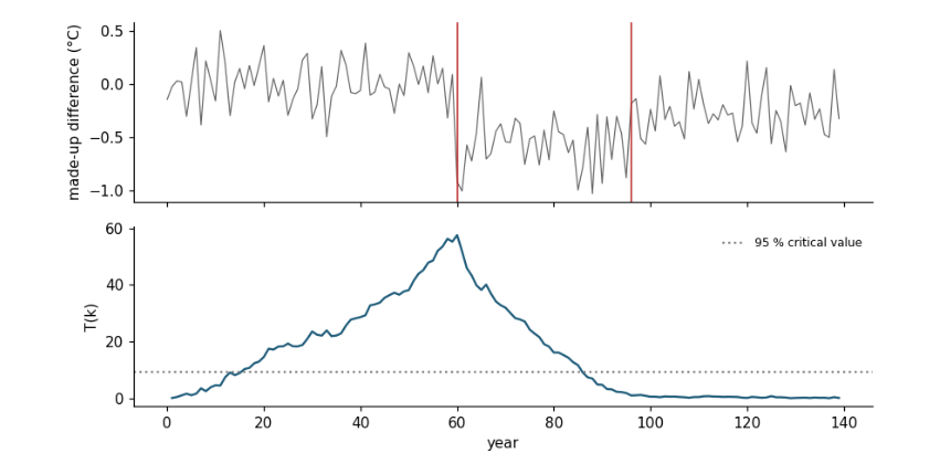
Reading it: the top panel is the made-up series with the detected breaks (red lines). The bottom panel is \(T(k)\) for the whole series: it peaks at the largest step, far above the dotted critical value.
Applying it to real stations
For each of our 40 stations: find neighbours within 500 km in the raw monthly archive whose year-to-year changes correlate with the station's at 0.6 or more over at least 30 years; keep the best 10; average their anomalies into a reference; find breaks in station minus reference; and shift each earlier segment to the level of the latest.
stations = pd.read_fwf(open_member("qcu", ".inv"), colspecs=[(0, 11), (12, 20), (21, 30)], names=["id", "lat", "lon"]).set_index("id")


def anomalies(a, col="t"):
    base = a[a.year.between(1951, 1980)].groupby("id")[col].agg(["mean", "size"])
    base = base.loc[base["size"] >= 15, "mean"]
    a = a[a.id.isin(base.index)].copy()
    a["anom"] = a[col] - a.id.map(base)
    return a


pool = anomalies(raw).pivot(index="year", columns="id", values="anom").loc[1850:2024]
dpool = pool.diff()
plat, plon = np.deg2rad(stations.lat.reindex(pool.columns)).values, np.deg2rad(stations.lon.reindex(pool.columns)).values


def homogenise(y, lat, lon):
    lat, lon = np.deg2rad(lat), np.deg2rad(lon)
    dist = 6371 * np.arccos(np.clip(np.sin(lat) * np.sin(plat) + np.cos(lat) * np.cos(plat) * np.cos(plon - lon), -1, 1))
    near = pool.columns[(dist < 500) & (dist > 0)]
    dy = y.diff()
    cors = {nb: dy.corr(dpool[nb]) for nb in near if (dy.notna() & dpool[nb].notna()).sum() >= 30}
    nbs = [k for k, v in sorted(cors.items(), key=lambda kv: -kv[1]) if v >= 0.6][:10]
    if len(nbs) < 3:
        return y, [], None
    ref = pool[nbs].mean(axis=1)
    d = (y - ref).dropna()
    bk = find_breaks(d.values)
    adj = pd.Series(0.0, index=d.index)
    edges = [0] + bk + [len(d)]
    last = d.iloc[edges[-2]:].mean()
    for a, b in zip(edges[:-1], edges[1:]):
        adj.iloc[a:b] = last - d.iloc[a:b].mean()
    return y + adj.reindex(y.index).bfill().ffill(), [d.index[i] for i in bk], d


dan = anomalies(daily)
mine = {}
for sid, g in dan.groupby("id"):
    y = g.set_index("year").anom.loc[1850:2024]
    mine[sid], brk, d = homogenise(y, sample.loc[sid, "lat"], sample.loc[sid, "lon"])
mine = pd.DataFrame(mine)
print("homogenised", mine.shape[1], "stations")
homogenised 39 stations
One station in detail
Let us look at one US station: the difference from its neighbours, the breaks found, and the corrected record.
sid = next(s for s in mine.columns if s.startswith("US") and len(homogenise(dan[dan.id == s].set_index("year").anom.loc[1850:2024], sample.loc[s, "lat"], sample.loc[s, "lon"])[1]) >= 2)
y = dan[dan.id == sid].set_index("year").anom.loc[1850:2024]
yh, brk, d = homogenise(y, sample.loc[sid, "lat"], sample.loc[sid, "lon"])
fig, axs = plt.subplots(2, 1, figsize=(9, 5), sharex=True)
axs[0].plot(d.index, d, color="0.4", lw=0.8)
for b in brk:
    axs[0].axvline(b, color="#b91c1c", lw=1)
axs[0].set_ylabel("station − neighbours (°C)")
axs[1].plot(y.index, y, color="0.6", lw=0.9, label="raw")
axs[1].plot(yh.index, yh, color="#1f5c7a", lw=1.1, label="our homogenisation")
axs[1].set_ylabel("anomaly (°C)")
axs[1].legend(frameon=False, fontsize=8)
fig.suptitle(f"Station {sid}: breaks in {', '.join(map(str, brk))}", fontsize=10)
plt.tight_layout()
plt.show()
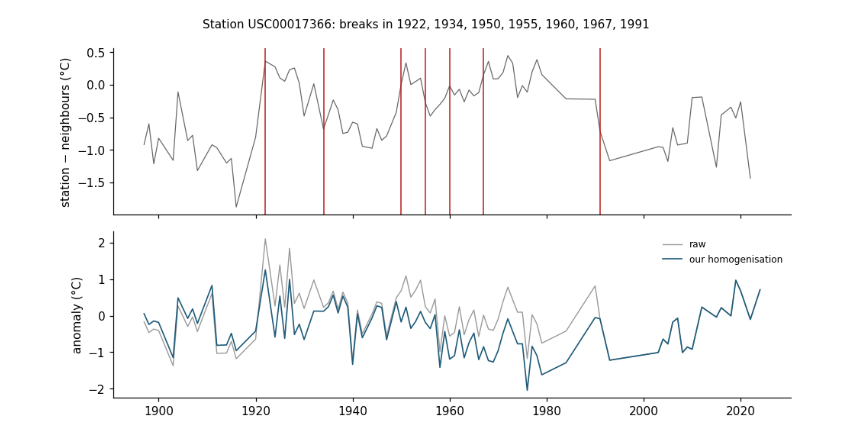
Reading it: the top panel is the station minus its neighbours; flat stretches separated by jumps are the signature of station changes, and the red lines mark the jumps found. In the bottom panel the corrected record (blue) is the raw one (grey) with each earlier stretch shifted by the size of its jump.
What neighbour methods cannot see
In the full analysis this method, applied to all of the study's stations, changes the US averages very little, while NOAA's corrections raise recent US warming considerably; outside the US our method and NOAA's agree. The reason is a limit of every neighbour comparison: it detects changes at one station relative to others. When almost every station in a region changes in the same years, the neighbours change too, and the difference series stays flat. That happened in the US: most volunteer observers moved their reading time from afternoon to morning over a few decades, and most switched to electronic sensors in the late 1980s. NOAA corrects these two with metadata (records of when each station changed) and physical models of their effect, not only with neighbours. An independent check is a different group's record: Berkeley Earth uses its own break detection and statistical method.
be = pd.read_csv(get("berkeley_conus.txt", "https://berkeley-earth-temperature.s3.us-west-1.amazonaws.com/Regional/TAVG/"
                     "contiguous-united-states-TAVG-Trend.txt"), comment="%", sep=r"\s+", header=None, usecols=[0, 1, 2],
                 names=["year", "month", "anom"]).dropna()
be = be.groupby("year").filter(lambda g: len(g) == 12).groupby("year").anom.mean()
us_mean = lambda frame: frame[[c for c in frame.columns if c.startswith("US")]].mean(axis=1)
wide = lambda a: a.pivot(index="year", columns="id", values="anom").loc[1850:2024]
rows = {"raw (our 20 US stations)": us_mean(wide(dan)),
        "our homogenisation": us_mean(mine),
        "NOAA homogenisation": us_mean(wide(anomalies(noaa[noaa.id.isin(pick)]))),
        "Berkeley Earth, whole contiguous US": be}
tab = pd.DataFrame({k: window_trends(v) for k, v in rows.items()}).T.round(3)
print(tab.drop(columns="1857-1898"))       # before 1899 only one or two of our 20 US stations report
1899-1940  1941-1982  1983-2024
raw (our 20 US stations)                 0.217     -0.193      0.157
our homogenisation                       0.151     -0.143      0.141
NOAA homogenisation                      0.227     -0.126      0.270
Berkeley Earth, whole contiguous US      0.165     -0.019      0.244
The first window is left out: before 1899 only one or two of these 20 stations report, so their average is not meaningful. Reading the table: compare the last column (1983-2024) down the rows. Our homogenisation changes the US stations little, while NOAA's raises recent warming. Berkeley Earth, made independently of NOAA, agrees with NOAA that recent US warming is faster than the raw stations show, and faster than 1899-1940.
7.4 The energy-balance model, 135 ways
The two-box model of the first notebook used one set of values: how much the climate eventually warms per unit of forcing (its sensitivity), how that warming splits between a fast and a slow box, and the two timescales. Here we vary all four over the ranges found in the literature and see whether the story of each period changes.
-
equilibrium sensitivity 2.0 to 4.5 °C for doubled CO₂ (a doubling is 3.93 W/m² of forcing);
-
fast share of the eventual warming 35 % to 55 %;
-
fast timescale 2 to 8 years; slow timescale 100 to 500 years.
f = pd.read_csv(DATA / "forcing.csv").rename(columns={"Unnamed: 0": "year"})
f["year"] = f.year.astype(int)
f = f.set_index("year").loc[:2024]
g = pd.read_csv(DATA / "hadcrut5.csv").rename(columns={"Time": "year", "Anomaly (deg C)": "global"}).set_index("year")["global"]


def respond(F, tau, q):
    out = np.zeros(len(F))
    for t_, q_ in zip(tau, q):
        box, a = 0.0, np.exp(-1 / t_)
        for i, x in enumerate(F):
            box = box * a + q_ * x * (1 - a)
            out[i] += box
    return pd.Series(out, index=F.index)


causes = {"greenhouse gases and other": f.anthro - f.aerosol, "aerosols": f.aerosol, "solar": f.solar, "volcanic": f.volcanic}
results = []
for ecs in (2.0, 2.5, 3.0, 3.5, 4.5):
    for share in (0.35, 0.45, 0.55):
        for tf in (2, 4, 8):
            for ts in (100, 250, 500):
                q = (share * ecs / 3.93, (1 - share) * ecs / 3.93)
                parts = {k: respond(v, (tf, ts), q) for k, v in causes.items()}
                fit = sum(parts.values())
                fit += (g - fit).loc[1850:2024].mean()
                resid = (g - fit).loc[1850:2024]
                row = {"ecs": ecs, "share": share, "tau_fast": tf, "tau_slow": ts,
                       "R2": 1 - (resid ** 2).sum() / ((g.loc[1850:2024] - g.loc[1850:2024].mean()) ** 2).sum()}
                for a, b in [(1910, 1945), (1946, 1975), (1976, 2024)]:
                    for k, v in parts.items():
                        row[f"{k} {a}-{b}"] = trend(v.loc[a:b].index, v.loc[a:b].values)
                    row[f"unexplained {a}-{b}"] = trend(resid.loc[a:b].index, resid.loc[a:b].values)
                results.append(row)
ebm = pd.DataFrame(results)
print(len(ebm), "versions; R² from", round(ebm.R2.min(), 2), "to", round(ebm.R2.max(), 2))
print(ebm.sort_values("R2").tail(3)[["ecs", "share", "tau_fast", "tau_slow", "R2"]])
good = ebm[ebm.R2 >= ebm.R2.quantile(0.75)]
print("\nrange over the best-fitting quarter of versions (°C/decade):")
print(good.filter(like="-").agg(["min", "max"]).T.round(3))
135 versions; R² from 0.35 to 0.91
    ecs  share  tau_fast  tau_slow        R2
78  3.0   0.55         8       100  0.907551
84  3.5   0.35         4       100  0.908231
87  3.5   0.35         8       100  0.910312

range over the best-fitting quarter of versions (°C/decade):
                                        min    max
greenhouse gases and other 1910-1945  0.050  0.075
aerosols 1910-1945                   -0.037 -0.021
solar 1910-1945                       0.004  0.006
volcanic 1910-1945                    0.008  0.018
unexplained 1910-1945                 0.097  0.114
greenhouse gases and other 1946-1975  0.092  0.133
aerosols 1946-1975                   -0.122 -0.084
solar 1946-1975                      -0.000  0.004
volcanic 1946-1975                   -0.017 -0.002
unexplained 1946-1975                -0.017  0.007
greenhouse gases and other 1976-2024  0.191  0.286
aerosols 1976-2024                   -0.034  0.013
solar 1976-2024                      -0.005 -0.002
volcanic 1976-2024                    0.015  0.025
unexplained 1976-2024                -0.082  0.008
Reading it: the best-fitting versions explain about 91 % of the variance, close to the single version used before. Over the best-fitting quarter, greenhouse gases supply most of the 1976-2024 warming, aerosols cancel most of the mid-century greenhouse warming, and the unexplained part of 1910-1945 stays at about 0.1 °C per decade. Even over all 135 versions, including poorly fitting ones, the unexplained early warming stays between about 0.07 and 0.14. The conclusions do not hang on the chosen timescales.
fig, axs = plt.subplots(1, 3, figsize=(12, 3.6))
for ax, per_ in zip(axs, ["1910-1945", "1946-1975", "1976-2024"]):
    cols = [c for c in ebm.columns if c.endswith(per_)]
    ax.boxplot([ebm[c] for c in cols], widths=0.6, showfliers=False)
    ax.set_xticks(range(1, len(cols) + 1))
    ax.set_xticklabels([c.replace(" " + per_, "").replace("greenhouse gases and other", "GHG +\nother") for c in cols], fontsize=7)
    ax.axhline(0, color="0.5", lw=0.8)
    ax.set_title(per_, fontsize=10)
axs[0].set_ylabel("contribution (°C per decade)")
plt.tight_layout()
plt.show()
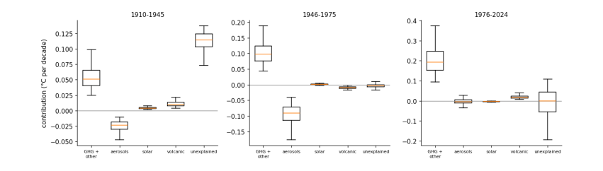
Reading it: a box plot summarises many values: the box spans the middle half, the line inside is the median, and the whiskers reach the range. One panel per period, one box per cause, across all 135 versions.
7.5 Many runs of one model
A climate model run with slightly different starting weather produces a different sequence of El Niños and ocean swings, while the forcing is identical. Comparing several runs of one model therefore measures chance in that model's climate. We read 10 runs each of two models from the cloud. As explained in notebook 2, a chunk that fails to download is silently filled with missing values, so we insist that every grid cell is present and retry otherwise.
import xarray as xr

cat = pd.read_csv(get("pangeo-cmip6.csv", "https://storage.googleapis.com/cmip6/pangeo-cmip6.csv"))
q_ = cat[cat.experiment_id.isin(["historical", "ssp245"]) & (cat.table_id == "Amon") & (cat.variable_id == "tas")]


def global_mean(store, tries=4):
    for k in range(tries):
        ds = xr.open_zarr(store.replace("gs://", "https://storage.googleapis.com/"), consolidated=True)
        w = np.cos(np.deg2rad(ds.lat))
        s = ds.tas.weighted(w).mean(("lat", "lon"), skipna=False).groupby("time.year").mean(skipna=False).to_series()
        if s.notna().all():
            return s
        time.sleep(5)
    raise RuntimeError("incomplete download")


runs = {}
for model in ("MIROC6", "CanESM5"):
    have = sorted(set(q_[(q_.source_id == model) & (q_.experiment_id == "historical")].member_id)
                  & set(q_[(q_.source_id == model) & (q_.experiment_id == "ssp245")].member_id),
                  key=lambda m: int(m[1:].split("i")[0]))[:10]
    for mem in have:
        cache = DATA / f"cmip6_{model}_{mem}.csv"
        if not cache.exists():
            sel = q_[(q_.source_id == model) & (q_.member_id == mem)]
            parts = [global_mean(sel[sel.experiment_id == e].sort_values("version").zstore.iloc[-1]) for e in ("historical", "ssp245")]
            pd.concat([parts[0], parts[1][parts[1].index > parts[0].index.max()]]).loc[1850:2024].to_csv(cache)
        s = pd.read_csv(cache, index_col=0).iloc[:, 0]
        runs[(model, mem)] = s - s.loc[1850:1900].mean()
runs = pd.DataFrame(runs)
tr = pd.DataFrame({k: window_trends(runs[k]) | {"1910-1945": trend(np.arange(1910, 1946), runs[k].loc[1910:1945].values)} for k in runs.columns}).T
print(tr.groupby(level=0).agg(["min", "max"]).round(3).T)
print("\nruns in which 1983-2024 is the fastest of the four windows:", int((tr[[f"{a}-{b}" for a, b in WINDOWS]].idxmax(axis=1) == "1983-2024").sum()), "of", len(tr))
CanESM5  MIROC6
1857-1898 min   -0.057  -0.040
          max    0.036   0.024
1899-1940 min    0.052   0.043
          max    0.123   0.085
1941-1982 min   -0.012  -0.040
          max    0.046   0.031
1983-2024 min    0.360   0.168
          max    0.486   0.220
1910-1945 min    0.047   0.048
          max    0.134   0.107

runs in which 1983-2024 is the fastest of the four windows: 20 of 20
fig, ax = plt.subplots(figsize=(9, 3.6))
for (model, mem), colr in zip(runs.columns, ["#ef4444"] * 10 + ["#2563eb"] * 10):
    ax.plot(runs.index, runs[(model, mem)].rolling(5, center=True).mean(), color=colr, lw=0.7, alpha=0.7)
ax.plot(g.index, (g - g.loc[1850:1900].mean()).rolling(5, center=True).mean(), color="k", lw=1.4, label="observed")
ax.plot([], [], color="#ef4444", label="MIROC6, 10 runs"); ax.plot([], [], color="#2563eb", label="CanESM5, 10 runs")
ax.set(ylabel="anomaly from 1850-1900 (°C), 5-yr mean")
ax.legend(frameon=False, fontsize=8)
plt.tight_layout()
plt.show()
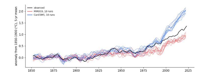
Reading it: runs of one model (one colour) share the forcing and the model's physics; they differ only by chance, and the spread between them is the size of chance. The two models differ more from each other than their runs do (CanESM5 is known to be one of the most sensitive models). In every run the last window warms fastest; the early window varies between runs by several hundredths of a degree per decade, which is how much an unlucky or lucky sequence of ocean swings can add.
7.6 Every window, not just four
The study chose four 42-year windows. A heat map shows the trend for every start year (horizontal) and every window length from 20 to 60 years (vertical); colour is the trend.
L, S0 = np.arange(20, 61), np.arange(1850, 2006)
M = np.full((len(L), len(S0)), np.nan)
for i, n in enumerate(L):
    for j, a in enumerate(S0):
        if a + n - 1 <= 2024:
            M[i, j] = trend(np.arange(a, a + n), g.loc[a:a + n - 1].values)
fastest_end = [int(S0[np.nanargmax(M[i])] + n - 1) for i, n in enumerate(L)]
print("for every window length from 20 to 60 years, the fastest window ends in:", sorted(set(fastest_end)))

fig, ax = plt.subplots(figsize=(9, 3.8))
im = ax.pcolormesh(S0, L, M, cmap="RdBu_r", vmin=-0.3, vmax=0.3, shading="nearest")
for a, b in WINDOWS:
    ax.plot(a, 42, "ko", ms=4)
ax.set(xlabel="first year of window", ylabel="window length (years)")
fig.colorbar(im, ax=ax, label="trend (°C per decade)")
plt.tight_layout()
plt.show()
for every window length from 20 to 60 years, the fastest window ends in: [2019, 2020, 2024]
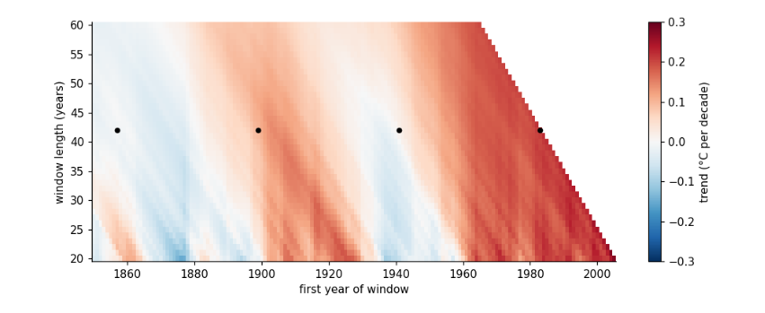
Reading it: red is warming, blue cooling; the black dots are the study's four windows. The deepest red is always at the right-hand edge, in windows that end in the last few years, whatever the length. The early-twentieth-century band is visible as a pale red stripe starting around 1900-1915, but it never reaches the colour of the recent band.
7.7 What this notebook adds
Shortcut removed |
What changed |
Does recent warming stay the fastest? |
|---|---|---|
Daily instead of monthly data |
Per-station trends are identical; the daily archive loses non-US stations after 2010 |
Yes, once stations are weighted by area |
Own homogenisation |
Finds about four breaks per station; fixes isolated changes, not network-wide ones |
Yes outside the US; for the US, NOAA and Berkeley Earth agree it does |
energy-balance versions |
Contributions vary in size, not in sign or ordering |
Yes |
Ten runs per model |
Chance moves early trends by a few hundredths |
Yes, in every run |
Every window |
Any start year, any length from 20 to 60 years |
Yes |
7.8 Recording what the run used
import json
print(json.dumps({"numpy": np.__version__, "pandas": pd.__version__, "xarray": xr.__version__,
                  "daily_stations": len(pick), "minutes": round((time.time() - t_start) / 60, 1)}, indent=1))
{
 "numpy": "2.0.1",
 "pandas": "2.2.3",
 "xarray": "2025.4.0",
 "daily_stations": 40,
 "minutes": 0.8
}
7.9 Where to go next
-
Run the homogenisation on all 1,155 of the study’s stations (about ten minutes) and compare US and non-US averages.
-
Add a metadata step: NOAA’s station-history database (HOMR) records when US cooperative observers changed their reading time; use it to correct the change from afternoon to morning readings and see how much of NOAA’s adjustment it explains.
-
Try a different break test (for example a penalised likelihood or the Pettitt test) and compare the breaks found.