5. Figures and records
5.1 Making and reading the figures
A figure answers a question only if you can say what each part shows. Before reading any chart, name its parts: what one mark is (a year, a bar), which column of the table goes on the x axis and which on the y axis, and in what units; what colour encodes; and whether uncertainty is shown.
fig, ax = plt.subplots(figsize=(8, 3.6))
ax.plot(d.year, d["global"], color="0.45", lw=1, label="Observed, global (HadCRUT5)")      # x: column 'year', y: column 'global'
ax.plot(m.year, m.model, color="#1f5c7a", lw=2, label="Model: response to all forcings")    # y: column 'model'
for (a, e), col in zip(WINDOWS, ["#ca8a04", "#64748b", "#b91c1c"]):                          # one trend line per window
    w = d[d.year.between(a, e)]
    k = np.polyfit(w.year, w["global"], 1)
    ax.plot(w.year, np.polyval(k, w.year), color=col, lw=2.5)
ax.set(xlabel="Year", ylabel="Anomaly (°C, vs 1961–1990)", title="Global temperature, the model, and three window trends")
ax.legend(frameon=False, fontsize=8)
plt.tight_layout()
plt.show()
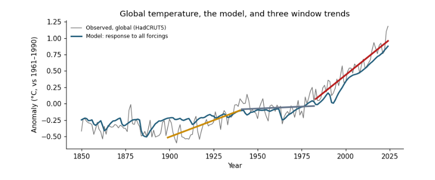
Reading it: the x axis is the year column; the y axis is the anomaly in °C. Each point on the grey line is one row of the table. The coloured segments are the three window trends from the trend table: the red one, 1983–2024, is the steepest. The blue line is the model, which knows nothing of the observed temperatures except their average level, yet follows the long rise, the dips after volcanic eruptions and the mid-century flat period.
fig, ax = plt.subplots(figsize=(7, 3.4))
split.set_index("period")[[*causes, "unexplained"]].plot.bar(ax=ax, width=0.8,
    color=["#b91c1c", "#64748b", "#ca8a04", "#0f766e", "#cbd5e1"])
ax.scatter(range(len(split)), split["global"], color="k", zorder=3, label="observed trend")
ax.axhline(0, color="0.5", lw=0.8)
ax.set(xlabel="", ylabel="Trend (°C per decade)", title="What drove each period's trend")
ax.legend(frameon=False, fontsize=8)
plt.xticks(rotation=0)
plt.tight_layout()
plt.show()
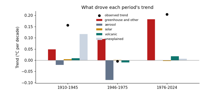
Reading it: one group of bars per row of the split table; one bar per cause column; the height is that cause's trend in °C per decade, below zero for cooling. The black dot is the observed trend; the bars in each group add up to it.
5.2 Recording what the run used
Good practice is to record what each run used: the versions of the libraries, the size of the data, and the time it took. Then anyone can see what they need to repeat it, and you can compare when the work grows.
record = {"python_packages": {"numpy": np.__version__, "pandas": pd.__version__},
          "data_files_mb": {p.name: round(p.stat().st_size / 1e6, 2) for p in sorted(DATA.glob("*.csv"))},
          "rows_in_joined_table": len(d),
          "result": {"global_trend_1983_2024": round(float(unc.trend.iloc[2]), 3), "global_trend_1899_1940": round(float(unc.trend.iloc[0]), 3)}}
print(json.dumps(record, indent=1))
{
 "python_packages": {
  "numpy": "2.0.1",
  "pandas": "2.2.3"
 },
 "data_files_mb": {
  "conus.csv": 0.0,
  "forcing.csv": 0.1,
  "hadcrut5.csv": 0.01,
  "owid_co2.csv": 14.38
 },
 "rows_in_joined_table": 175,
 "result": {
  "global_trend_1983_2024": 0.216,
  "global_trend_1899_1940": 0.101
 }
}
5.3 Where to go next
-
Change a window in
WINDOWSand rerun: does the ordering of trends change? -
Replace the global series with the US one in the energy-balance section: how much more does a single region vary?
-
Read the essay Reading climate data for what these results mean, and the guide Hypothesis testing with climate data for the statistics in depth.